Fig. 1.
Synoptic maps at 0000 UTC 05 June 2008 for nature run (a) and control run (b). The wind barbs denote the wind fields at 50 m AGL. Shaded contour represents the wind speeds. The contours show the temperature at 700 hPa pressure level (2°C interval). The thick black line denotes the cold front. The large box denotes the key front region, that is, used for calculations in Figs. 12, 17, 19 and 20. The small box denotes the key LLJ region used for the calculation in Fig. 12.
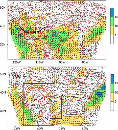
Fig. 2.
Distribution of surface observation stations (plus signs) and terrain heights (shaded contour; unit: m). The two solid dots denote the locations of the two stations in single station experiments.
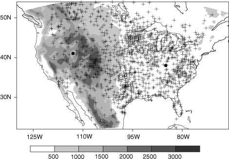
Fig. 3.
The 3DVAR analysis increments of temperature (K; top row), u-component (m s−1; middle row) and v-component (m s−1; bottom row) of wind at the lowest model level with assimilation of 2-m temperature (left column), 10-m winds (middle column) and both 2-m temperature and 10-m winds (right column) from a single observation station over complex terrain. The shaded contours show the terrain heights (unit: m). ‘+' denotes the location of the observation station.
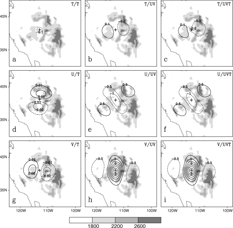
Fig. 4.
Same as Fig. 3, except over flat terrain.
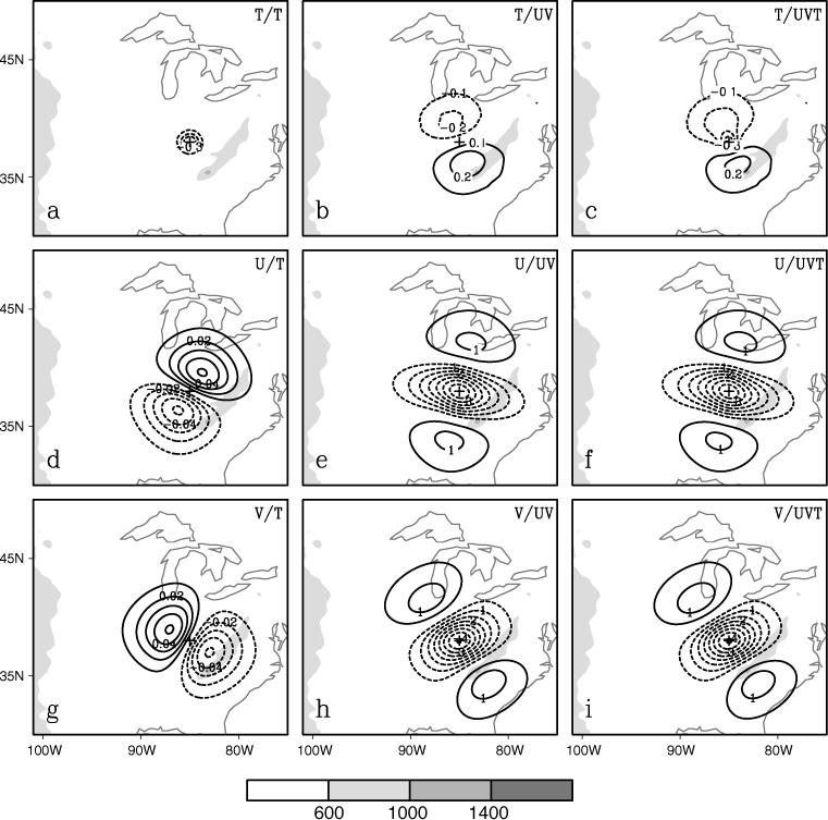
Fig. 5.
Schematic illustration of the correlation and cross-correlation functions for multivariate OI analysis derived using the geostrophic increment assumption (courtesy Gustafsson 1981 and Kalnay 2003). ‘φ’ is thermodynamic variable related to the temperature. u and v denote the horizontal components of wind.
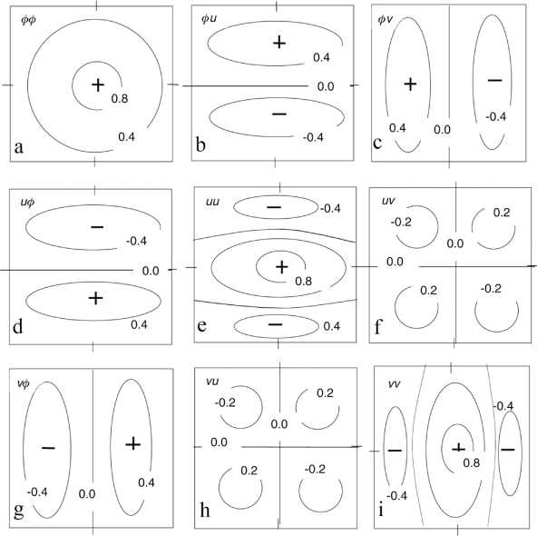
Fig. 6.
The 3DVAR analysis increments of temperature (K) with assimilation of both 2-m temperature and 10-m winds from a single observational station over complex terrain using different horizontal correlation length-scales: a default value (middle), 25% of the default value (left) and 150% of the default value (right). The shaded contour shows the terrain heights (m).
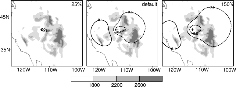
Fig. 7.
Same as Fig. 3, except for the EnKF analysis increments. The half radius of the horizontal localization used in the experiments is 320km. No vertical localization is applied.
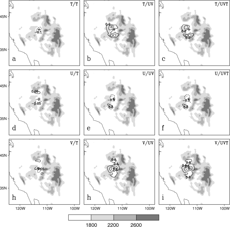
Fig. 8.
Same as Fig. 7, except over flat terrain.
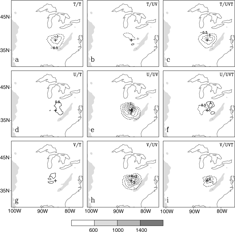
Fig. 9.
Ensemble spread (shaded) and analysis increments (contour) for temperature (a; 0.1 K interval), u-component (b; 0.2 m s−1 interval) and v-component (c; 0.2 m s−1 interval) with assimilation of both 2-m temperature and 10-m wind using EnKF. The ‘+’ sign denotes the observational location.
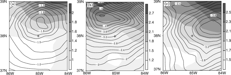
Fig. 10.
Same as Fig. 6, except for EnKF with different radii of horizontal localization. The default value of half radius of the horizontal localization is 320 km (middle). The smaller (left) and larger (right) scales are 20% and 200% of the default value, respectively.
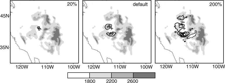
Fig. 11.
Estimated background error standard deviation of the streamfunction (shaded contour; unit: 105 m2 s−1) in 3DVAR (a, static in time) and EnKF [b, averaged over the data assimilation period (0000 UTC to 0600 UTC 5 June 2008)] near 800 m AGL. Contour lines denote the terrain heights (interval: 500m).
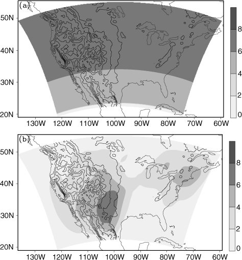
Fig. 12.
Time-height root-mean-square errors (against the nature run) of temperature (K; left column) averaged over a key front region and wind speed (m s−1; right column) averaged over a key LLJ region, for EnKF experiments with various maximum radii of vertical localization scales: 1000m (a and b), 3000m (c and d), 5000m (e and f). The key frontal region and the key LLJ region are marked in Fig. 1b.
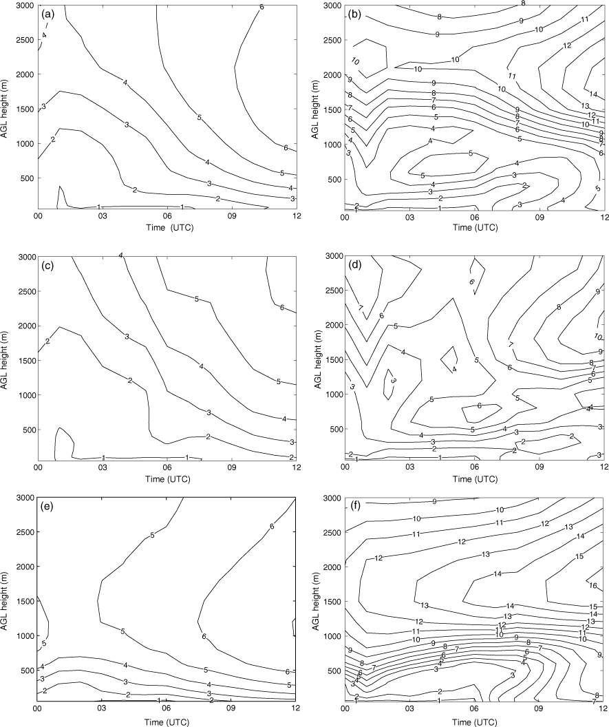
Fig. 13.
Same as Fig. 1, except for the 3DVAR (a) and EnKF (b) analysis after the first data assimilation cycle.
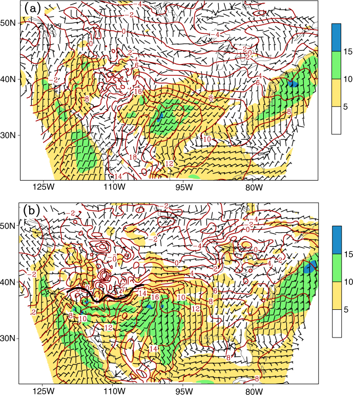
Fig. 14.
Same as Fig. 1, except for 0600 UTC 05 June 2008 for nature run (a), control run (b), 3DVAR analysis (c), and EnKF analysis (d).
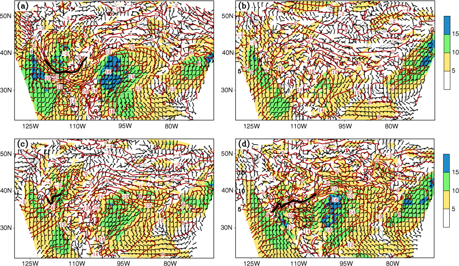
Fig. 15.
Vertical profiles of mean wind speed (m s−1) over the key regions of LLJ. Over a box of (32°N–38°N; 103°W–97°W) after the first data assimilation cycle at 0000 UTC 5 June 2008 (a), (28°N–38°N; 103°W–95°W) at the end of data assimilation cycle at 0600 UTC 5 June 2008 (b), and (32°N–40°N; 105°W–95°W) after 6 h forecast at 1200 UTC 5 June 2008 (c).
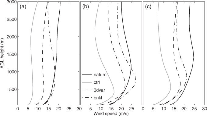
Fig. 16.
Time-latitude cross-section of temperature averaged over the main front zone in 6° longitude ranging from 114°W to 108°W at 500 m AGL for nature run (a), control run (b), 3DVAR analysis (c), and EnKF analysis (d). The dashed bold lines denote the cold front.
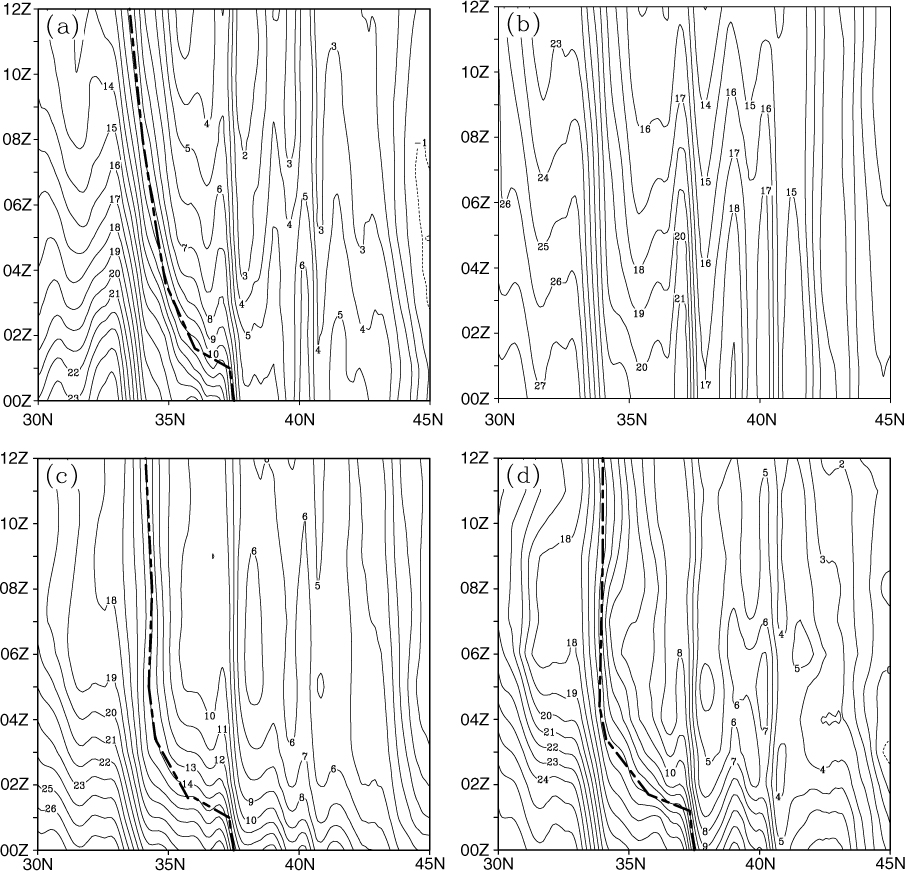
Fig. 17.
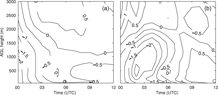
The time-height differences of the root-mean-square (RMS) errors (against the nature run) between EnKF and 3DVAR for (a) temperature (K) and (b) wind speed (m s−1), calculated over all stations in the key front region as marked in Fig. 1b. The negative numbers imply EnKF has smaller RMS errors, relative to 3DVAR.
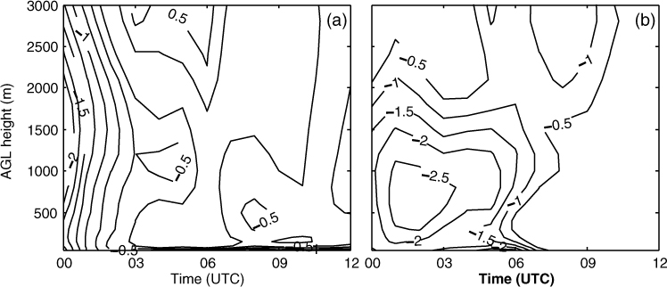
Fig. 18.
Same as Fig. 2, except triangle signs denote rejected stations.
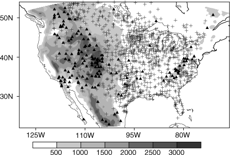
Fig. 19.
Time-height root-mean-square (RMS) errors (against the nature run) of temperature (K; left column) and wind speed (m s−1; right column) for EnKF analysis and subsequent forecast in the key front region as marked in Fig. 1b. For the default experiment without terrain perturbation and data rejection (a and b); RMS error differences between the experiment with terrain perturbation and default experiment (c and d; positive numbers denote the degraded analysis and forecast from the experiment with terrain perturbation); and the RMS error differences between the experiment with data rejection and the default experiment (positive numbers mean the degraded analysis and forecast from the data rejection experiment).
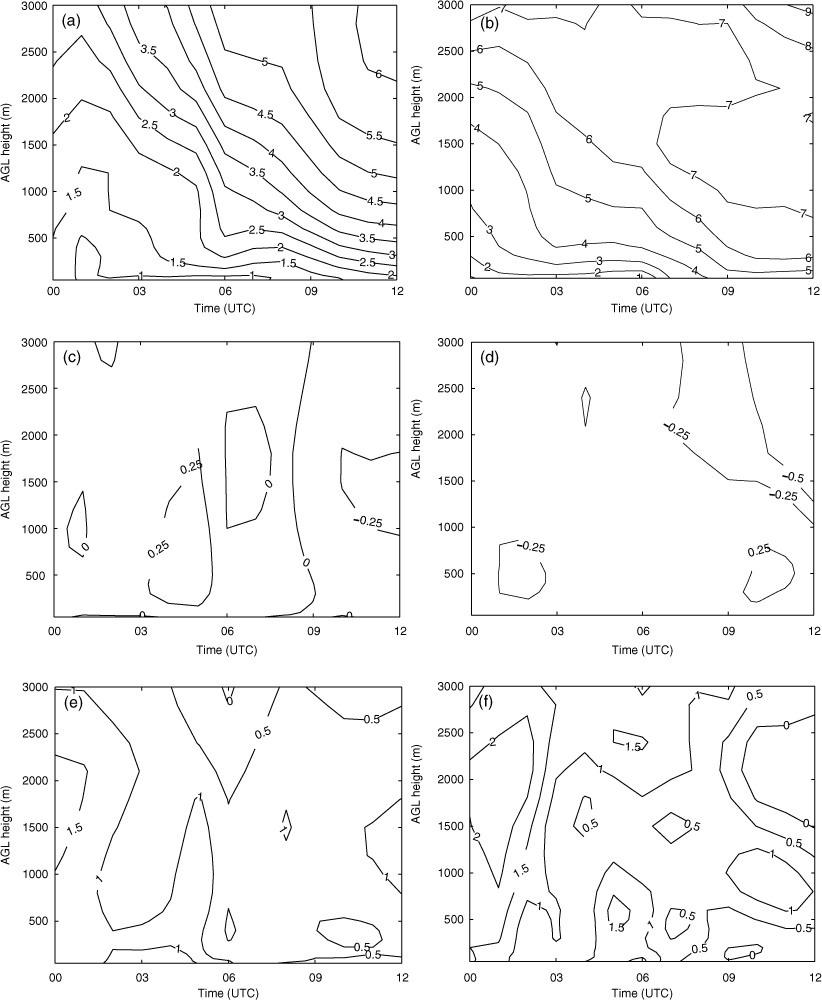
Fig. 20.
Same as Fig. 17, except for the data rejection experiment.