Fig. 1.
Initial state: meridional cross-section at the position of the potential vorticity anomaly. Displayed are zonal wind (black contours, from 5 m s−1 to 35 m s−1), isentropes (gray, every 5 K) and the 2-pvu tropopause (green). Colors show the perturbation of the zonal wind by the initial potential vorticity anomaly in intervals of 2.5 m s−1 with blue indicating easterly and red westerly winds.
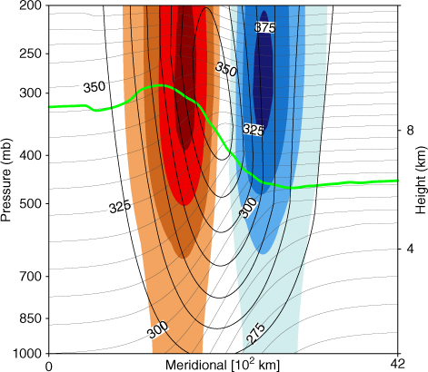
Fig. 2.
Time evolution of the baroclinic wave at day 0 (a), day 2 (b), day 4 (c) and day 6 (d). Shown are vertically averaged kinetic energy (dashed, contours for 100, 300, 500 and 700 J m−3) and pressure advection v a ·∇ h p* (color). The green contour indicates the 2-pvu isoline on 320 K and gray solid contours depict surface potential temperature (every 6 K).
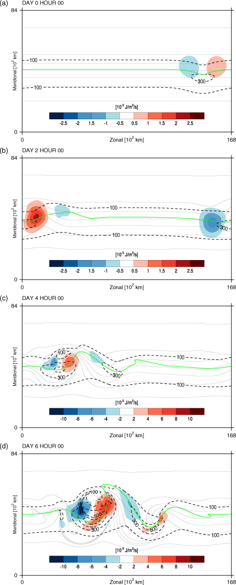
Fig. 3.
Synoptic evolution of the downstream cyclone: incipient frontal cyclone (a), late frontal fracture (b), and T-bone stage (c). Surface potential temperature (black solid, every 4 K), surface pressure (dashed, every 10 hPa), surface wind speeds (brown, contours from 20 m s−1 in steps of 5 m s−1 with areas above 35 m s−1 dotted) and 2-pvu isoline on 320 K (green).
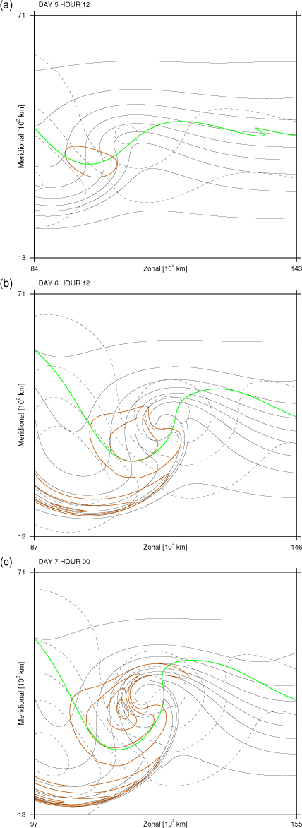
Fig. 4.
Initiation of the lower-tropospheric cyclone. Shown in (a) are upper-level divergence of ageostrophic geopotential fluxes ∇·(p*u a ) (color) and kinetic energy (dashed, contrours for 100, 300 and 500 J m−3) at a height of 6 km as well as the 2-pvu isoline on 320 K (green). Potential temperature at the surface is shown by gray, solid lines (every 6 K). Panel (b) shows baroclinic conversion (color) at 2 km height and kinetic energy at the surface (dashed, contours for 100, 300 and 500 J m−3). Also shown are surface pressure (thin dashed, every 5 hPa) and potential temperature (gray solid, every 6 K). The location of strongest downward motion at a height of 2 km is indicated by the −0.0075 m s−1 contour of the vertical wind (green).
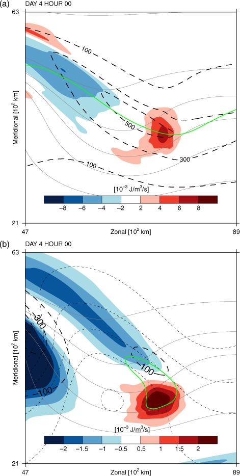
Fig. 5.
(a) Evolution of kinetic energy, (b) baroclinic conversion and (c) ageostrophic geopotential flux divergence along 1.5 d trajectories ending at day 4 hour 12 in the low-level KE center (KE ≥100 J m−3) and a height between 100 and 500 m. The target area on the lowest model level is schematically depicted in the upper left corner of (a). The trajectories are divided in two categories depending on whether the divergence of ageostrophic geopotential fluxes is positive (red) or negative (blue) at day 4 hour 12. The standard deviation (±σ) within each category is indicated by the shading. Note the different scales used in (b) and (c).
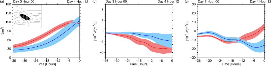
Fig. 6.
Redistribution of kinetic energy due to the ageostrophic circulation. (a) shows the divergence of ageostrophic geopotential fluxes ∇·(p*ua ) (color) at the surface and the −8 J m−2 s−1 isoline of vertical ageostrophic geopotential fluxes at 2 km (blue) at day 5. (b) shows the divergence of ageostrophic geopotential fluxes (color) and horizontal ageostrophic geopotential flux vectors with a magnitude greater than 3000 J m−2 s−1 at day 6. Also shown are surface fields of KE (dashed, contours for 100, 200, 300 and 400 J m−3), pressure (thin dashed, every 5 hPa) and potential temperature (solid gray, every 6 K). The cross-hatched symbol shows the location of the surface pressure minimum.
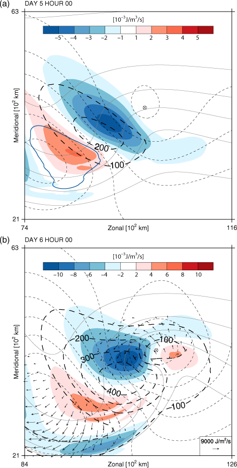
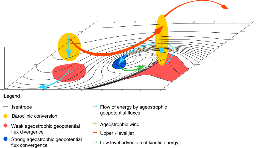
Fig. 7.
Schematic of the horizontal ageostrophic circulation and ageostrophic geopotential fluxes associated with a circular, eastward propagating lower-tropospheric cyclone L and an anticyclone H. Depicted are (a) the low-level ageostrophic circulation and its decomposition into isallobaric and advective component and (b) horizontal ageostrophic geopotential fluxes and their divergence and convergence pattern.
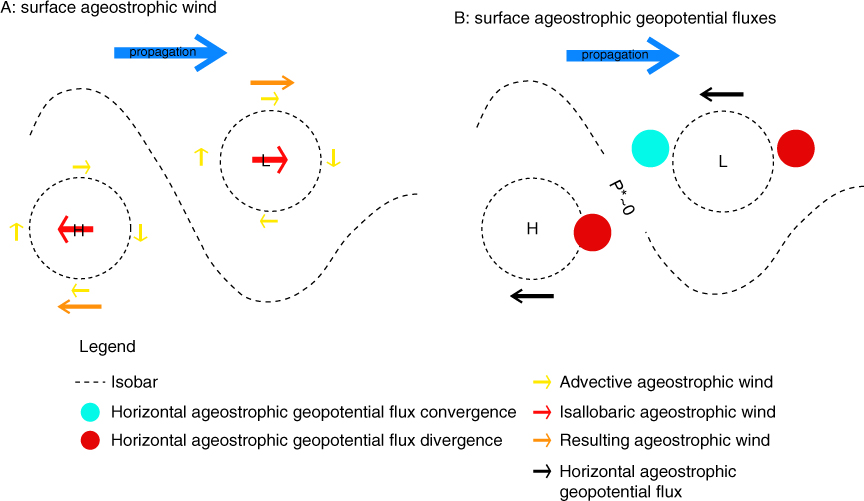
Fig. 8.
(a) Surface isallobaric and (b) advective wind contributions to (c) the total ageostrophic wind. Background fields are surface potential temperature (solid, every 6 K) and pressure (dashed, every 5 hPa).
Fig. 9.
Same as Fig. 6a but for vertical ageostrophic geopotential fluxes at 2 km at day 5. Note the different scales for downward (blue) and upward (red) fluxes.
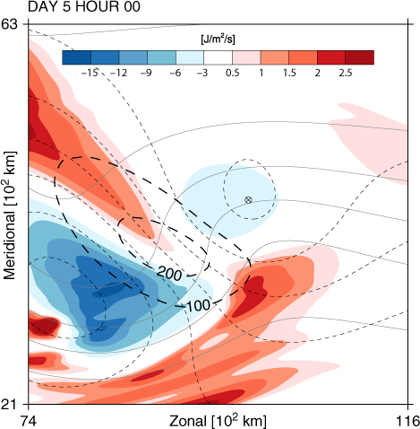
Fig. 10.
Formation of the low-level jet at day 6 hour 18. Shown are divergence of ageostrophic geopotential fluxes ∇·(p*u a ) (color), horizontal ageostrophic geopotential flux vectors p*va greater than 6000 J m−2 s−1, and kinetic energy (dashed, for 300, 600, 900 and 1200 J m−3) at the surface. Downward ageostrophic geopotential fluxes at a height of 2 km are indicated by the −20 J m−2 s−1 contour (blue) and upward fluxes by the 10 J m−2 s−1 contour (red). The background fields are surface pressure (thin dashed, every 10 hPa) and surface potential temperature (solid gray, every 6 K). The cross-hatched symbol shows the location of the surface pressure minimum.
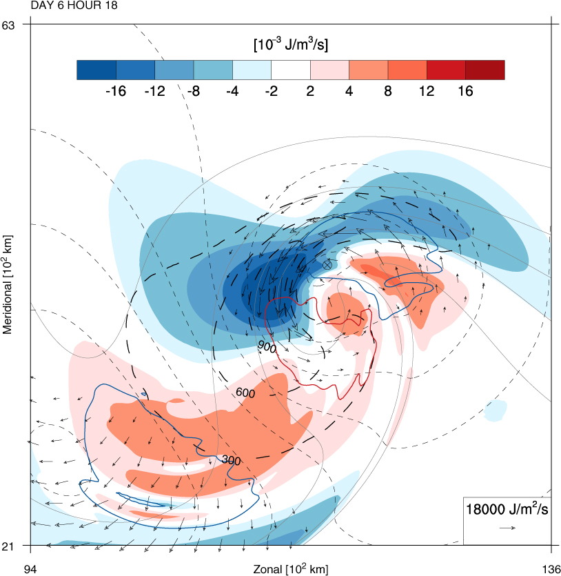
Fig. 11.
Panel (a) shows a section across the downstream cyclone in the T-bone stage at day 6 hour 18 with divergence of ageostrophic geopotential fluxes ∇·(p*u a ) (color), kinetic energy (dashed, every 200 J m−3 from 300 J m−3) and potential temperature (gray solid, every 4 K). The location of the cross-section is shown in (b). J1 denotes the southward jet, J2 the northward jet, CF the cold front, WF the warm front and BF the bent-back front. Panel (b) is the same as Fig. 10 but with advection of kinetic energy vG ·∇ h E K (color).
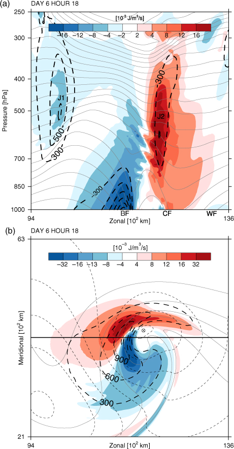
Fig. 12.
(a) Evolution of kinetic energy, (b) baroclinic conversion and (c) divergence of ageostrophic geopotential fluxes along 2 d trajectories arriving at day 6 hour 18 in the low-level jet (KE ≥900 J m−3). Panel (a) shows the subset of trajectories located at the northern boundary of the 900 J m−3 contour of KE (dashed) at day 6 hour 18, and colors indicate KE at the midpoint of each line segment. Black dots denote the position of every trajectory at day 6 hour 18. Surface pressure (thin dashed, every 10 hPa) and potential temperature (solid, every 10 K) at day 6 hour 18. Note the different scales used in (b) and (c). The shading represents the standard deviation ±σ.
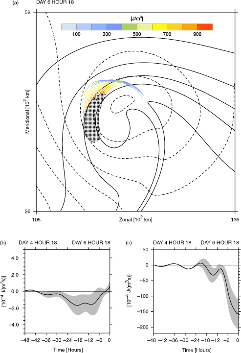
Fig. 13.
Schematic summarizing the generation of KE in the lower troposphere by baroclinic conversion and its redistribution by ageostrophic geopotential fluxes and advection in an idealised downstream cyclone.