
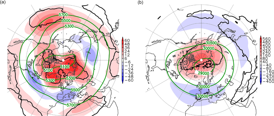
Fig. 1
ERA-Interim geopotential height differences (gpm) between low (2001–2012) and high (1980–2000) ice period for winter (DJF) in (a) 500 hPa and (b) 10 hPa. Green contours show the climatological mean (1980–2012), black contours the 90% confidence level calculated from a U test.
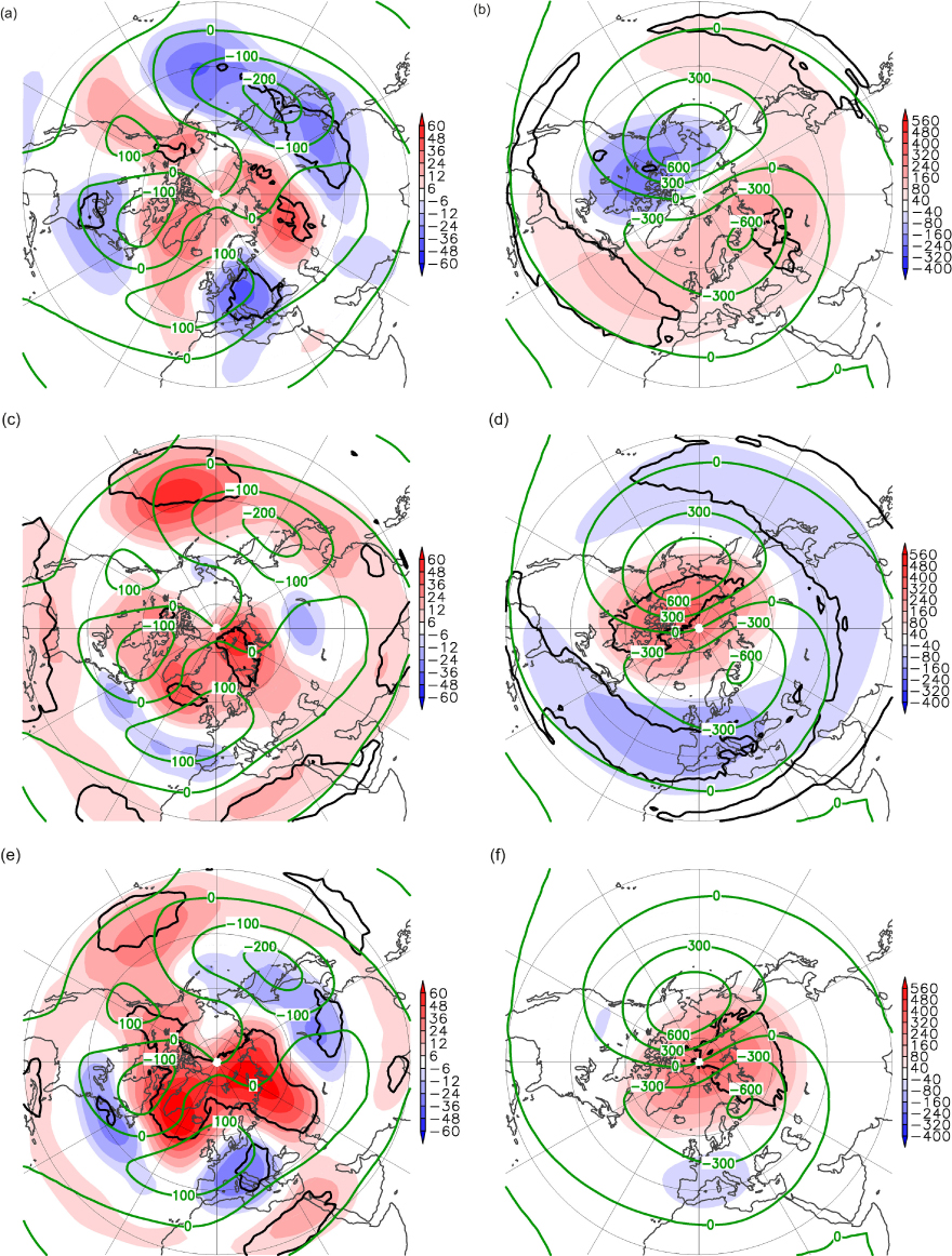
Fig. 2
ERA-Interim geopotential height differences (gpm) in (a, c, e) 500 hPa and (b, d, f) 10 hPa (a, b) between the 1980–1989 decade and the 1990–1999 decade, (c, d) between low ice period (2001–2012) and the 1980–1989 decade and (e, f) between low ice period (2001–2012) and the 1990–1999 decade for winter (DJF). Green contours show the climatological departures from the zonal mean (1980–2012), black contours the 90% confidence level calculated from a U test.
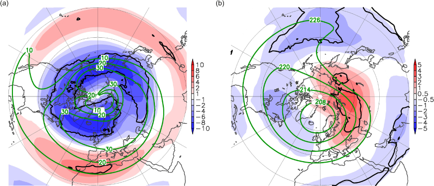
Fig. 3
ERA-Interim (a) zonal wind (m/s) and (b) temperature differences (K) between low (2001–2012) and high (1980–2000) ice period for winter (DJF) in 10 hPa. Green contours show the climatological mean (1980–2012), black contours the 90% confidence level calculated from an U test.
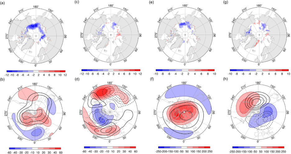
Fig. 4
First (a, b and e, f) and second pair (c, d and g, h) of coupled patterns obtained by the Maximum-Covariance-Analysis (MCA) of August/September HadISST1 sea ice concentration (1979–2011) and ERA-Interim winter (DJF) geopotential height fields (1980–2012). Upper row displays the sea ice concentration anomaly maps in percent as heterogeneous regression maps. Lower row contains the corresponding anomaly maps for geopotential heights in 500 hPa (b, d) and 10 hPa (f, h) in gpm, shown as homogeneous regression maps. Black contours in (b) and (f) show the climatological mean (1980–2012) with 5100 gpm, 5200 gpm, and 5300 gpm isolines in (b) and 29000 gpm, 30000 gpm, and 30500 gpm isolines in (f) starting from the pole. Black contours in (d) and (h) show the climatological departures from the zonal mean (1980–2012) with 50 gpm contour interval in (d) and 150 gpm contour interval in (h). Negative contours are dashed.
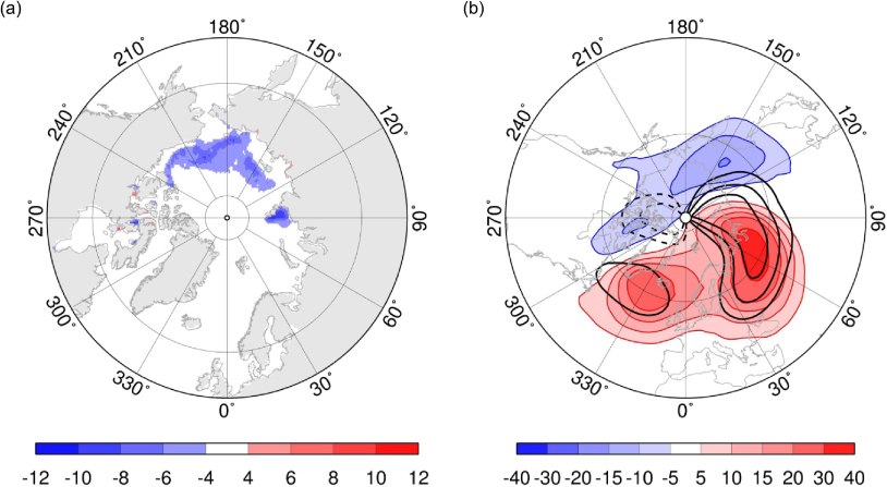
Fig. 5
First pair of coupled patterns obtained by the maximum covariance analysis of (a) August/September HadSST1 sea ice concentration (1979–2011) in percent displayed as heterogeneous regression map and (b) ERA-Interim winter (DJF) meridional heat flux on planetary scales (10–90 d) in 10 hPa (1980–2012) in Km/s displayed as homogeneous regression map. Black contour in (b) shows the climatological mean (1980–2012) with 20 Km/s contour interval. Negative isolines are dashed.
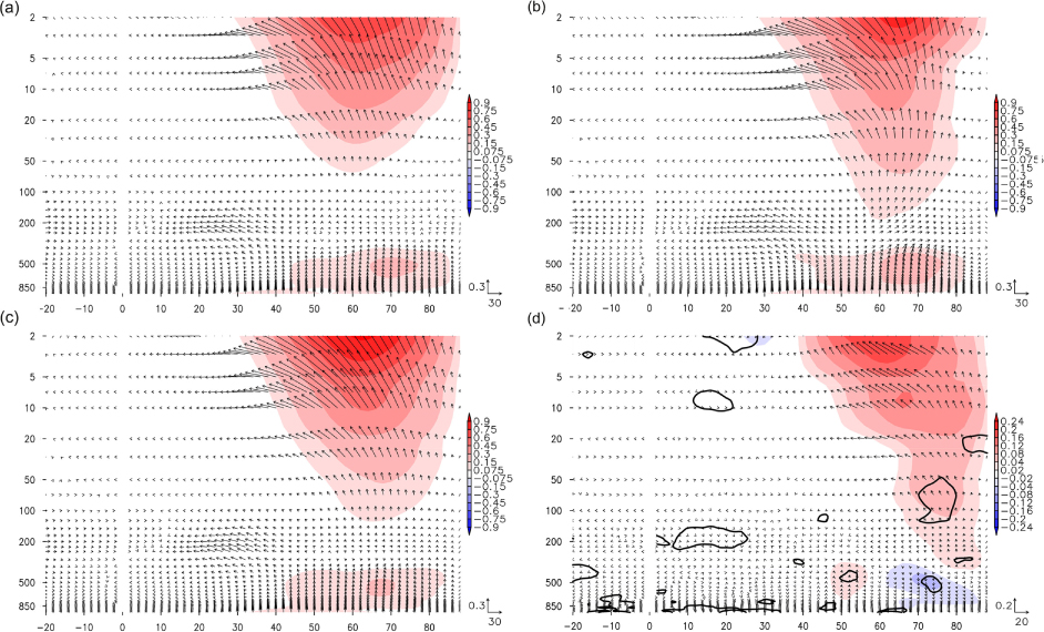
Fig. 6
Zonal mean ERA-Interim vertical component of EP flux (m2/s2, shaded) and vertical and meridional component (vectors) on planetary scales (10–90 d) for (a) the 1980–1989 decade (b) the 1990–1999 decade, (c) the low ice period (2001–2012) and (d) as differences between low (2001–2012) and high (1980–2000) ice phase for December. Black contours show the 90% confidence level calculated from a U test.
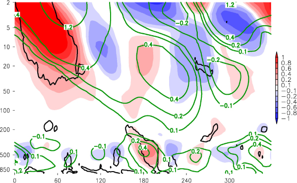
Fig. 7
ERA-Interim vertical component of EP flux vector differences (m2/s2) on planetary scales (10–90 d) between low (2001–2012) and high (1980–2000) ice period for December meridional mean cross-section between 66 and 80°N. Green contours show the climatological mean (1980–2012), black contours show the 90% confidence level calculated from a U test.