Fig. 1.
Synthetic 2-D turbulent flow. (a) RMSE between mean estimate of vorticity and ground truth; (b) RMSE between mean estimate of velocity and ground truth.
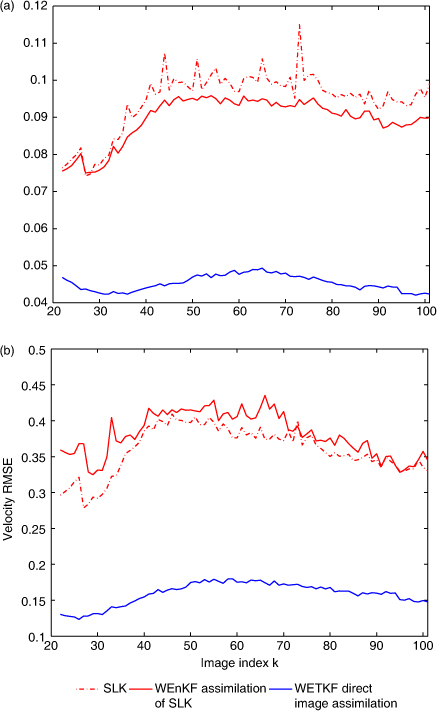
Fig. 2.
Synthetic 2-D turbulent flow. (a) Energy spectra; (b) error energy spectra.
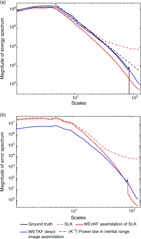
Fig. 3.
Synthetic 2-D turbulent flow. (a) Example of scalar image of the sequence at given time k; (b) ground truth vorticity at time k; (c) SLK vorticity estimate; (c) mean estimate of vorticity with WEnKF assimilation of SLK observation; (d) mean estimate of vorticity with WETKF direct assimilation of image data.
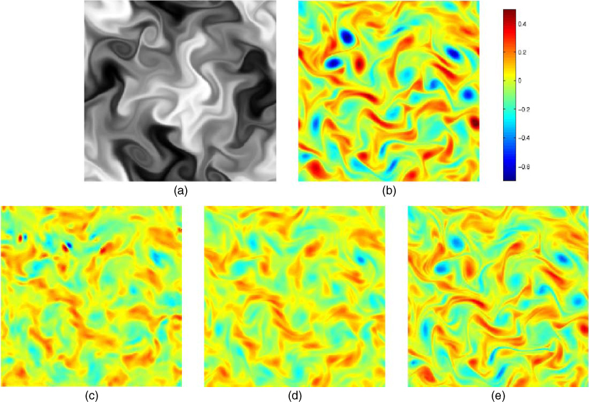
Fig. 4.
Comparison of WEnKF and WETKF techniques for the direct assimilation of image data. (a) RMSE between mean estimate of vorticity and ground truth; (b) RMSE between mean estimate of velocity and ground truth.
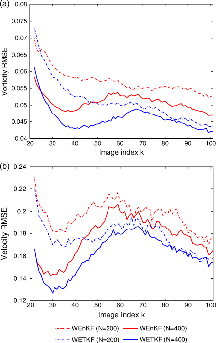
Fig. 5.
(a) Error Energy spectrum in log k vs. kE(k) scale obtained with ETKF (dotted lines) and WETKF (plain lines) for different number of particles; (b) Energy spectrum in log-log scale obtained with ETKF (dotted lines) and WETKF (plain lines) for different number of particles; (c) vorticity root-mean-square error along time obtained for WETKF with a diagonal constant observation variance (blue) and with the empirical image based variance (red).
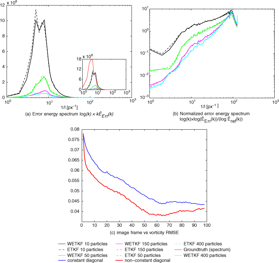
Table 1. Experiments on 2-D turbulence
[i] Results obtained from WEKF and ETKF are compared. For both filters the dynamic's noise has a standard deviation of 0.01 and the parameters of the self-similar power law are fixed from the ground truth data. Mean-square estimation errors with respect to the ground truth and the ensemble dispersion around the ground truth are indicated in the table. Note the ground truth is associated to a zero variance as it is a deterministic system. The mean has been computed through an empirical average over the 20 last image frames of 10 realisations.
Fig. 7.
Visualisation (with 50 members) of the covariance matrix values corresponding to the central line at t=99 left: ETKF, right: WETKF. The significative covariance length-scale is about 15×Δx large for both filters.
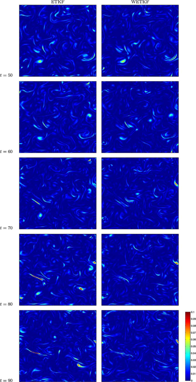
Fig. 8.
Left: visualisation for WETKF (with 400 members) of an example of the image-based adapted variance map associated to the displaced frame observation model; right: corresponding image of the passive scalar. High values of the standard deviation correspond to areas associated with high photometric gradient.
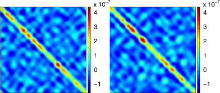
Fig. 6.
Example of the ensemble dispersion maps evolution along time; left column ETKF ensemble dispersion; right column WETKF ensemble dispersion.
Fig. 9.
Real 2-D turbulent flow (Jullien et al., 2000). (a) Image at given time k and estimated velocity field with SLK; (b) image at given time k and estimated velocity field with WEnKF assimilation of SLK result; (c) image at given time k and estimated velocity field with WETKF direct assimilation of image data; (d) vorticity estimate with SLK and associated velocity field; (e) mean estimate of vorticity with WEnKF assimilation of SLK observation, and associated velocity field; (f) mean estimate of vorticity with WETKF direct assimilation of image data, and associated velocity field; (g–i) zoom in on white delimited areas of (d–f).
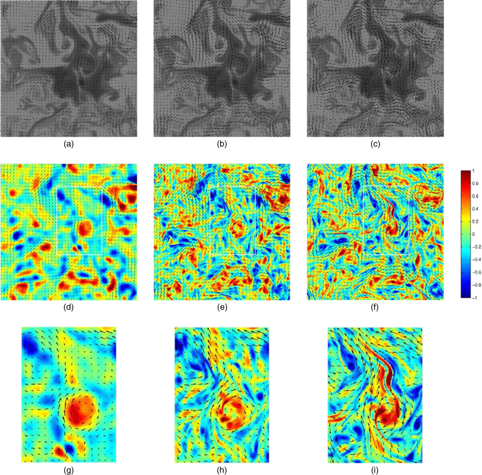
Fig. 10.
Synthetic oceanic sequence with missing data. (a) Image at given time k; (b) image at given time k+1; (c) Ground truth vorticity and velocity field; (d) mean estimate of vorticity and velocity from WETKF assimilation of images without missing data; (e) mean estimate of vorticity and velocity from WETKF assimilation of images with missing data shown in (a) and (b).
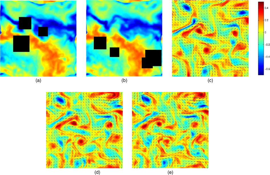
Fig. 11.
Synthetic oceanic sequence with missing data. (a) RMSE between mean estimate of vorticity and ground truth; (b) RMSE between mean estimate of velocity and ground truth.
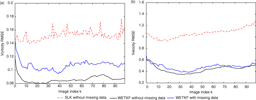
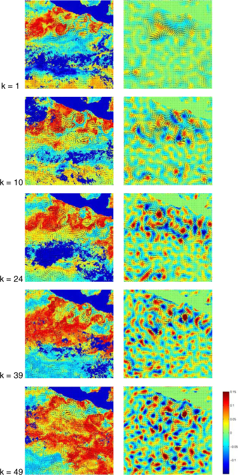
Fig. 12.
Real satellite sequence of SST (sea surface temperature) images. Dark blue regions indicate missing data due to the cloud cover or land regions. First column: SST images at different times k=1, 10, 24, 39, 49 and estimated velocity fields with the WETKF assimilation of image data. Second column: Mean estimated vorticity with WETKF and associated velocity fields.