Fig. 1.
The stream function and the corresponding quasi-geostrophic winds of the Ref-1 and Ref-2 basic flows adopted in Experiments I and II, respectively. (a) and (b) correspond to the Ref-1 basic flow; (c) and (d) correspond to the Ref-2 basic flow.
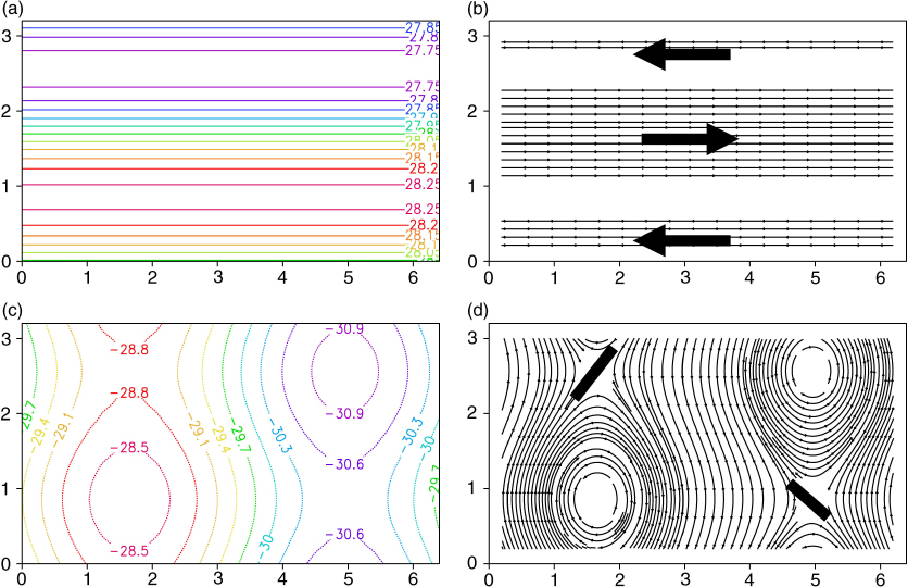
Fig. 2.
The stream function components of the NFSVs and FSVs of the Ref-1 basic flow with a perturbation magnitude of 1.6. The left (right) column lists the NFSVs (FSVs) with optimisation times of 2, 5, 7, and 9 d.
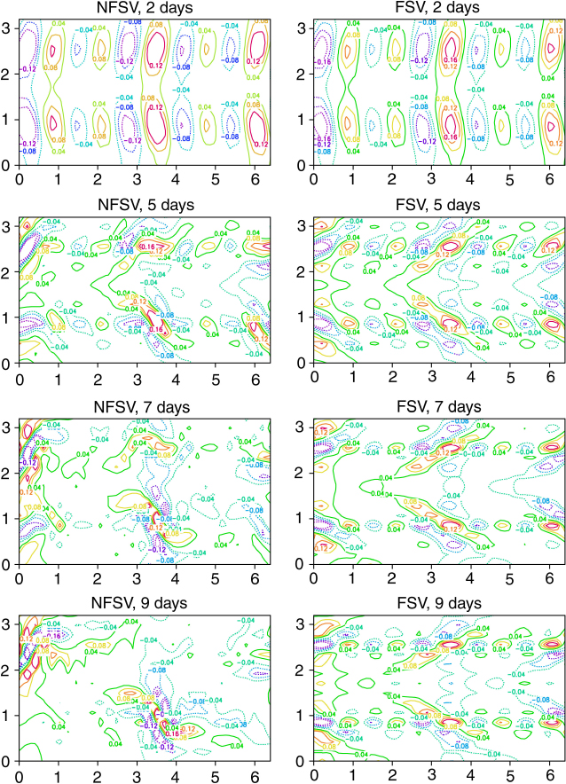
Fig. 3.
The stream function components of the Ref-1 NFSVs and FSVs with an optimisation time of 7 d. The left (right) column lists the NFSVs (FSVs) with perturbation magnitudes of 0.8, 1.6, 2.4, and 3.2.
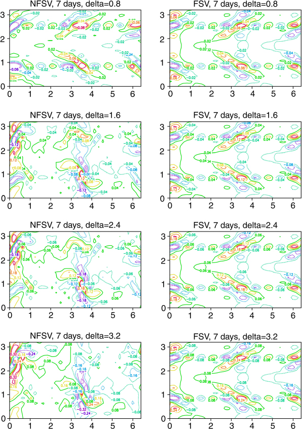
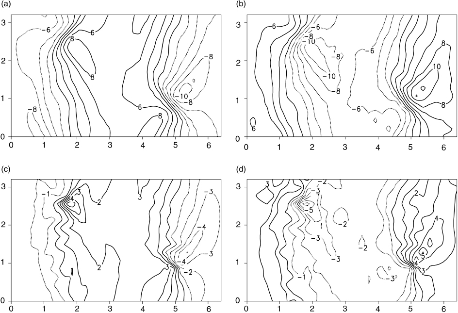
Fig. 4.
Patterns of the stream functions of the prediction errors caused by (a) the FSV in the linearised QG model, (b) the FSV in the non-linear QG model, and (c) the NFSV in the non-linear QG model, where the optimisation is 7 d and the model perturbation magnitude is 1.6 in terms of the chosen norm.
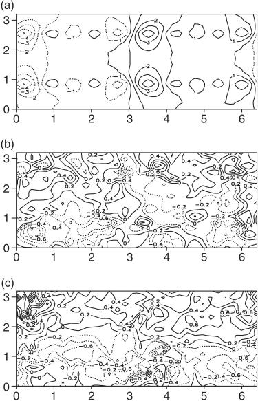
Fig. 5.
The prediction errors caused by the NFSVs and the FSVs in the QG model (denoted by NFSV-n and FSV-n) and those caused by the FSVs in the linearised QG model (denoted by FSV-l). The horizontal axis represents the perturbation magnitudes, and the vertical axis describes the prediction errors in terms of the energy. (a) uses an optimisation time of 2 d, and (b) uses the optimisation time of 7 d.
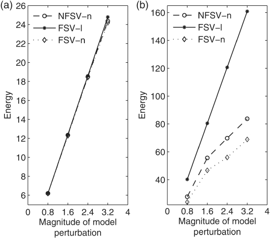
Fig. 6.
The zonal-means of the stream function of prediction errors (left column) and the corresponding zonal wind (right column) caused by (a, b) the FSV in the linearised QG model, (c, d) the FSV in the non-linear QG model, and (e, f) the NFSV in the non-linear QG model. The optimisation time is 7 d, and the model perturbation magnitude is 1.6.
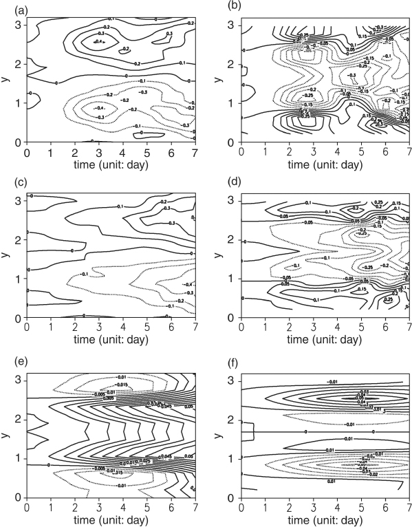
Fig. 7.
The stream function patterns of the prediction error caused by the tendency perturbation in the linearised QG model (left column) and the differences between the stream function induced by the tendency perturbation in the non-linear QG model and that in the linearised QG model (right column). The latter indicates the effect of non-linear advection on the perturbation growth. (a) and (b) are for the FSV, and (c) and (d) are for the NFSV. Both FSV and NFSV are computed with the optimisation time 7 d and the tendency perturbation magnitude 1.6. The figures in (a, b, c, and d) correspond to the patterns at the final time of optimisation time.
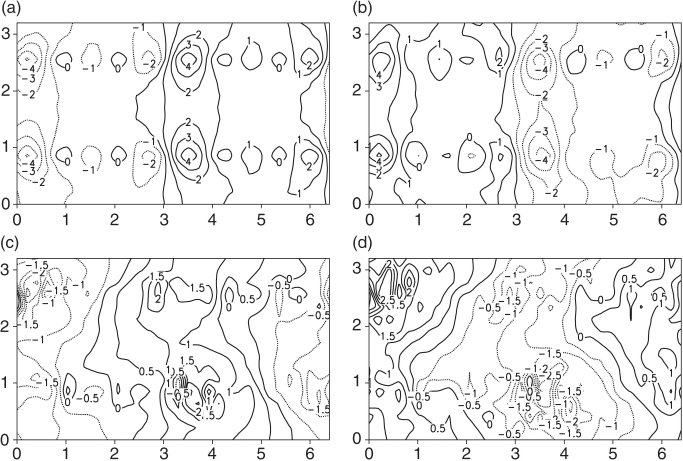
Fig. 8.
The stream function components of the Ref-2 NFSVs and FSVs with a perturbation magnitude of 1.6. The left (right) column lists the NFSVs (FSVs) with optimisation times of 2, 5, 7, and 9 d.
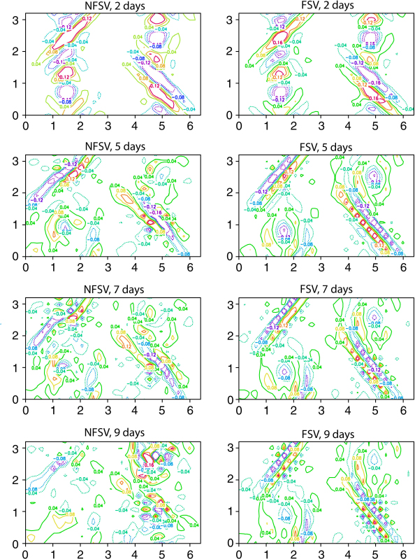
Fig. 9.
The stream function components of the Ref-2 NFSVs and FSVs with an optimisation time of 7 d. The left (right) column lists the NFSVs (FSVs) with model perturbation magnitudes of 0.8, 1.6, 2.4, and 3.2.
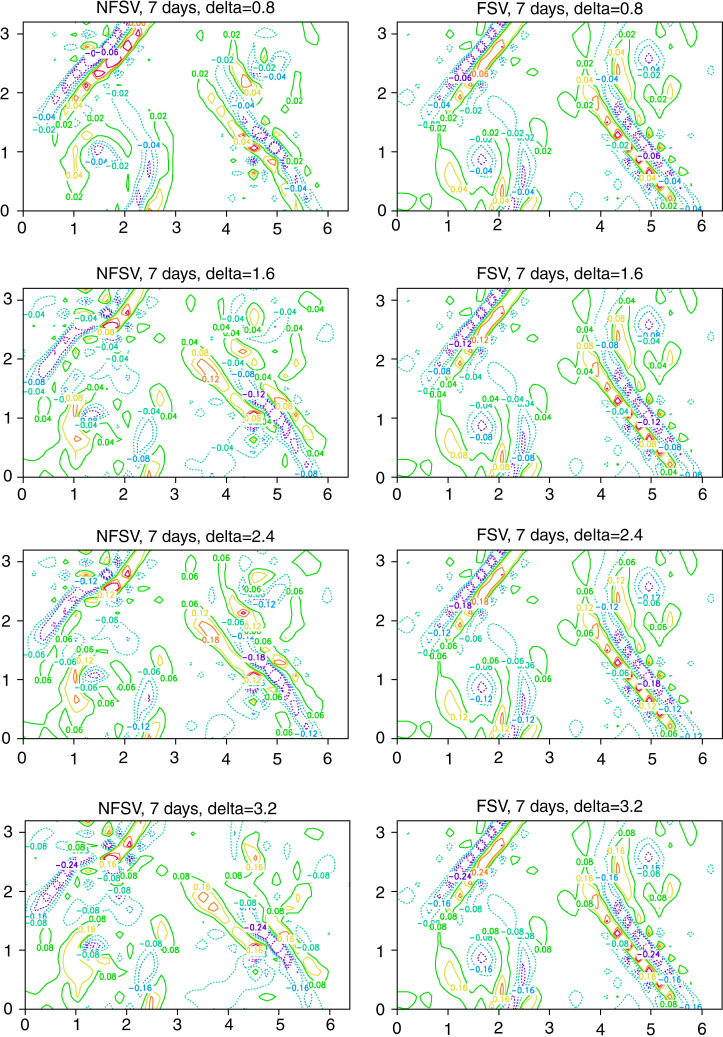
Fig. 10.
The prediction errors caused by the NFSVs and the FSVs in the QG model (denoted by NFSV-n and FSV-n) and those caused by the FSVs in the linearised QG model (denoted by FSV-l). The horizontal axis represents the perturbation magnitudes, and the vertical axis describes the prediction errors in terms of the energy. (a) uses an optimisation time of 2 d, and (b) uses an optimisation time of 7 d.
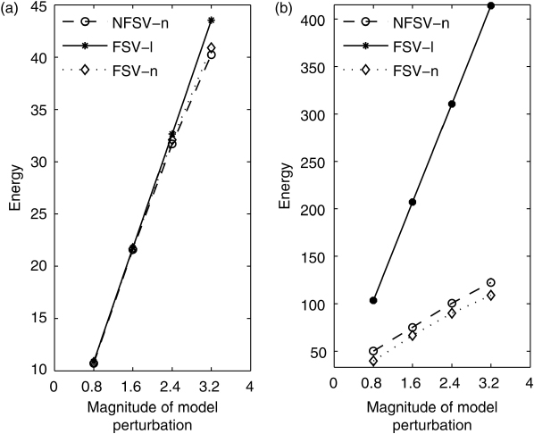
Fig. 11.
Patterns of the stream functions of the prediction errors caused by (a) the FSV in the linearised QG model, (b) the FSV in the non-linear QG model, and (c) the NFSV in the non-linear QG model, where the optimisation is 7 d and the model perturbation magnitude is 1.6 in terms of the chosen norm.
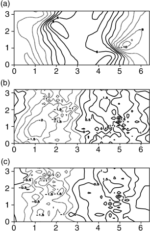
Fig. 12.
The meridional-mean of the stream function of prediction errors (left column) and the corresponding meridional wind (right column) caused by (a, b) the FSV in the linearised QG model, (c, d) the FSV in the non-linear QG model, and (e, f) the NFSV in the non-linear QG model. The optimisation time is 7 d, and the model perturbation magnitude is 1.6.
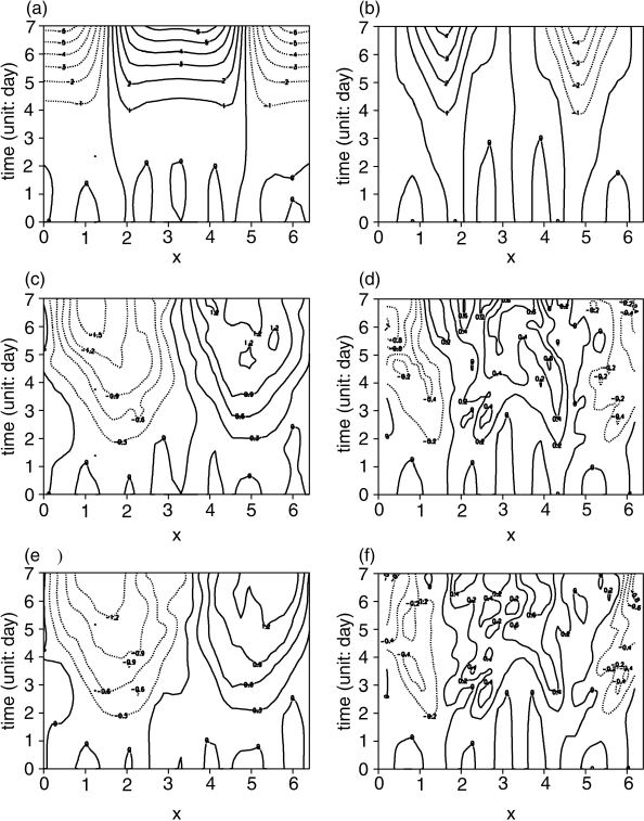
Fig. 13.
The patterns of the stream function of the prediction error caused by the optimal forcing in the linearised QG model (left column) and the differences between the perturbation stream function induced by the optimal forcing in the non-linear QG model and in the linearised QG model (right column). The latter indicates the non-linear effects of perturbation advection on the perturbation growth. (a) and (b) are for the FSV, and (c) and (d) are for the NFSV. Both the FSV and NFSV are computed with an optimisation time of 7 d and a model perturbation magnitude of 1.6.