
Table 1. Summary of information on the CMIP3 models used in this study. The abbreviations for each model are used throughout the paper
Fig. 1.
Teleconnection patterns determined by rotated EOF analysis of fields of Z 500 ERA40 re-analysis, DJF from 1958 to 1999. (a) PNA (13.7% explained variance), (b) NAO (12.8%), (c) EA (9.8%), (d) WP (7.9%), (e) EA/WR (7.8%), (f) POL (6.6%), (g) TNH (6.2%), (h) SCAN (6.0%), (i) EP/NP (5.7%). For explanations of abbreviations see Table 2.

Table 2. Summary of used abbreviations for teleconnection patterns
Fig. 2.
Taylor plots for NAO of fields of Z 500 CMIP3/AMIP3 model runs and NCEP/NCAR and ERA40 re-analysis, DJF. (a) CMIP3 from 1958 to 1999, (b) CMIP3/AMIP3 from 1979 to 1999.
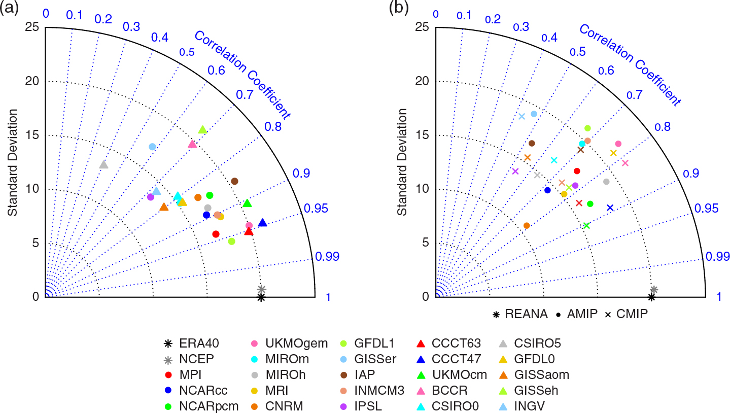
Fig. 3.
Taylor plots for EA of fields of Z 500 CMIP3/AMIP3 model runs and NCEP/NCAR and ERA40 re-analysis, DJF. (a) CMIP3 from 1958 to 1999, (b) CMIP3/AMIP3 from 1979 to 1999.
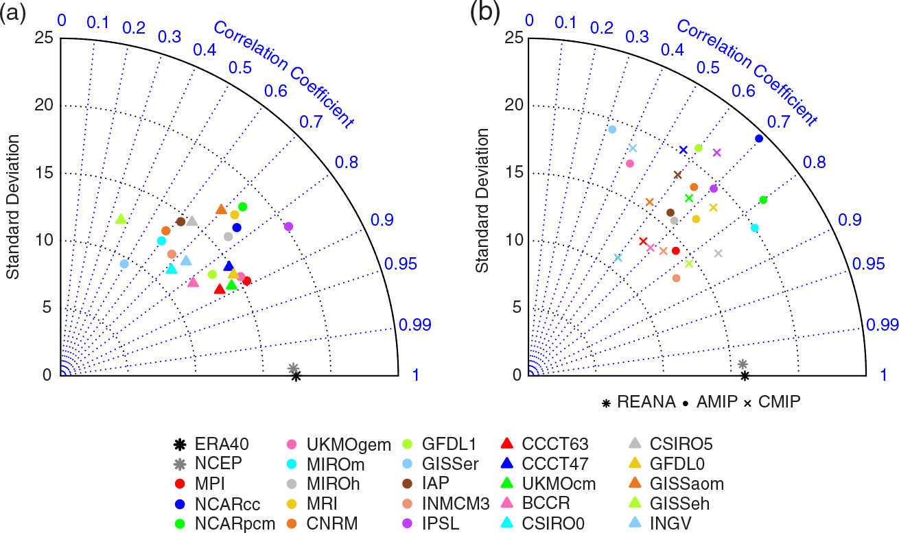
Fig. 4.
Taylor plots for PNA of fields of Z 500 CMIP3/AMIP3 model runs and NCEP/NCAR and ERA40 re-analysis, DJF. (a) CMIP3 from 1958 to 1999, (b) CMIP3/AMIP3 from 1979 to 1999.
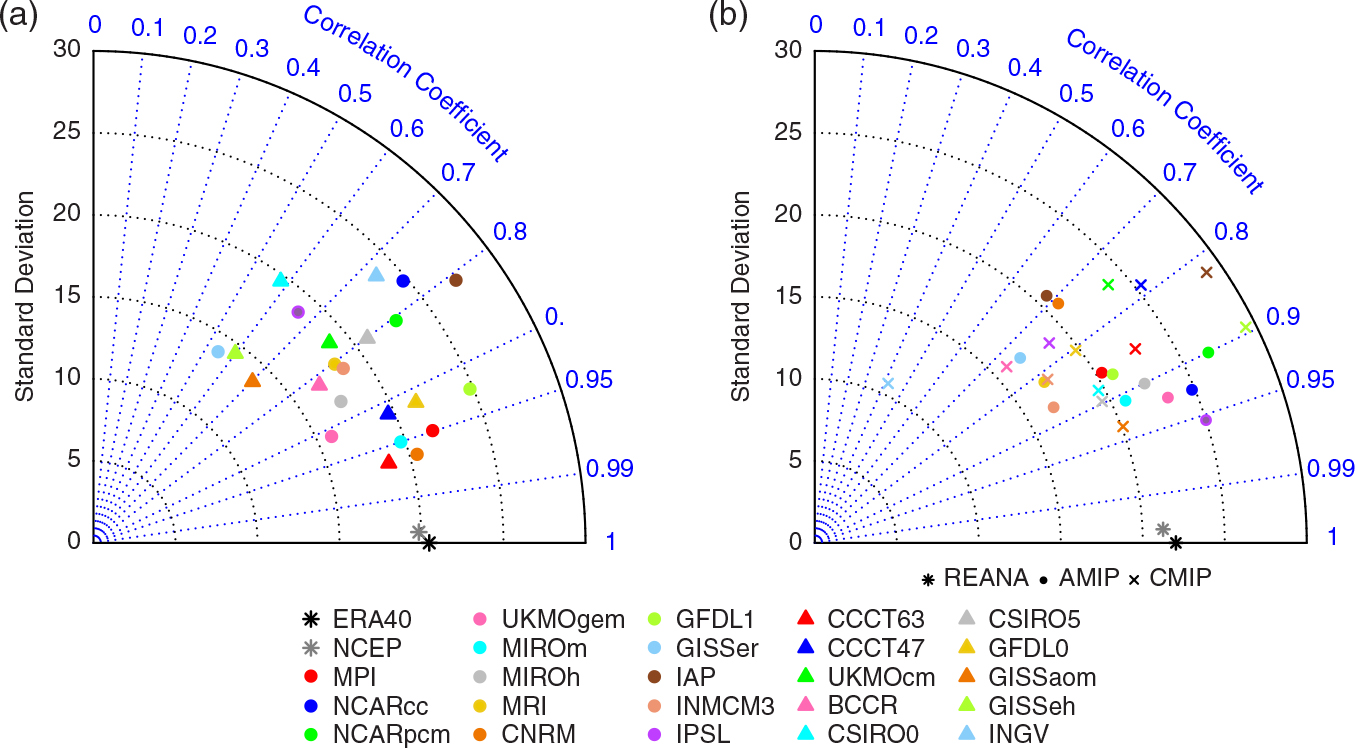
Fig. 5.
Taylor plots for WP of fields of Z 500 CMIP3/AMIP3 model runs and NCEP/NCAR and ERA40 re-analysis, DJF. (a) CMIP3 from 1958 to 1999, (b) CMIP3/AMIP3 from 1979 to 1999.
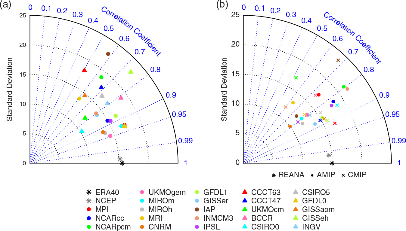
Fig. 6.
Taylor plots for the normalised pattern statistics within a multi-member ensemble of simulations of the NAO pattern at Z 500 for DJF, CMIP3 from 1958 to 1999. (a) Four-member ensemble of ECHAM5/MPI-OM1, (b) Eight-member ensemble of NCAR CCSM3.
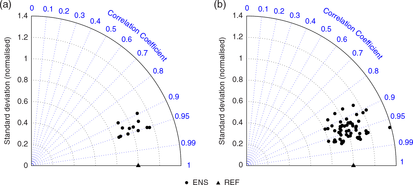
Fig. 7.
Taylor plots for the normalised pattern statistics within a multi-member ensemble of simulations of the PNA pattern at Z 500 for DJF, CMIP3 from 1958 to 1999. (a) four-member ensemble of ECHAM5/MPI-OM1, (b) eight-member ensemble of NCAR CCSM3.
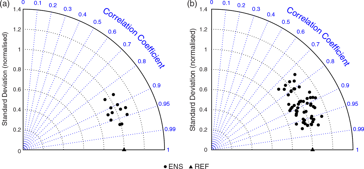
Table 3. Mean intra-ensemble correlations for all ensembles and all patterns. For abbreviations of models see Table 1
[i] Bold: Maximal attainable correlation.
Table 4. Skill score ranges (mean±standard deviation) for the multi-model ensemble of CMIP3 1958–1999, CMIP3 1979–1999 and AMIP3 1979–1999, respectively
Fig. 8.
Metric for teleconnection patterns of fields of Z 500, skill score S according to eq. (2). (a) CMIP3 from 1958 to 1999, all patterns, (b) AMIP3 and CMIP3 from 1979 to 1999, all patterns. In each rectangle the lower triangle gives the value for the AMIP3 run and the upper that of the CMIP3 run.
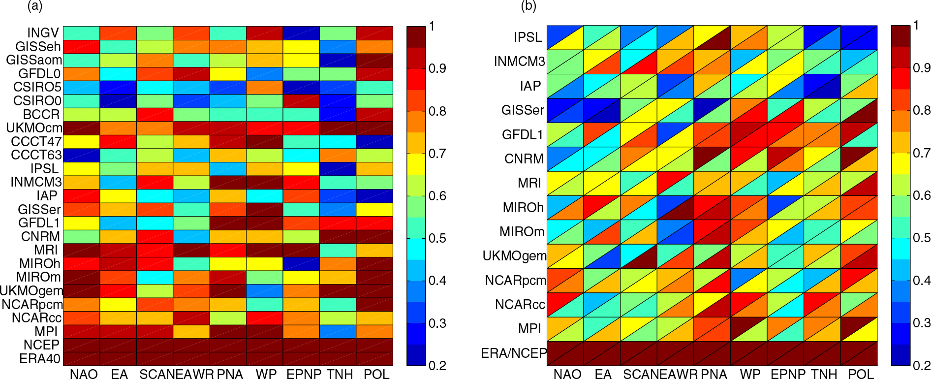
Fig. 9.
Wavelet power spectra of time-series of teleconnection patterns at Z 500. ERA40 re-analysis, DJF from 1958 to 1999. (a) NAO-index, (b) PNA-index. The wavelet transformation was performed with the Morlet wavelet. At both ends, dash-dotted lines separate regions where edge effects become important. The thick red contour envelopes areas of greater than 95% confidence for a corresponding red noise process with lag-one autocorrelation-coefficients of 0.19 (NAO) and 0.22 (PNA), respectively.
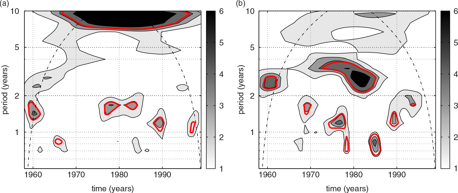
Fig. 10.
Wavelet power spectra of time-series of teleconnection patterns at Z 500. CMIP3 runs of ECHAM5/MPI-OM (a, b) and UKMO HadGEM1 (c, d), DJF from 1958 to 1999. (a, c) NAO-index, (b, d) PNA-index. For further explanations see Fig. 9. The corresponding red noise processes have lag-one autocorrelation-coefficients of 0.06 (NAO, ECHAM5/MPI-OM), 0.15 (PNA, ECHAM5/MPI-OM), 0.21 (NAO, UKMO HadGEM1) and 0.16 (PNA, UKMO HadGEM1), respectively.
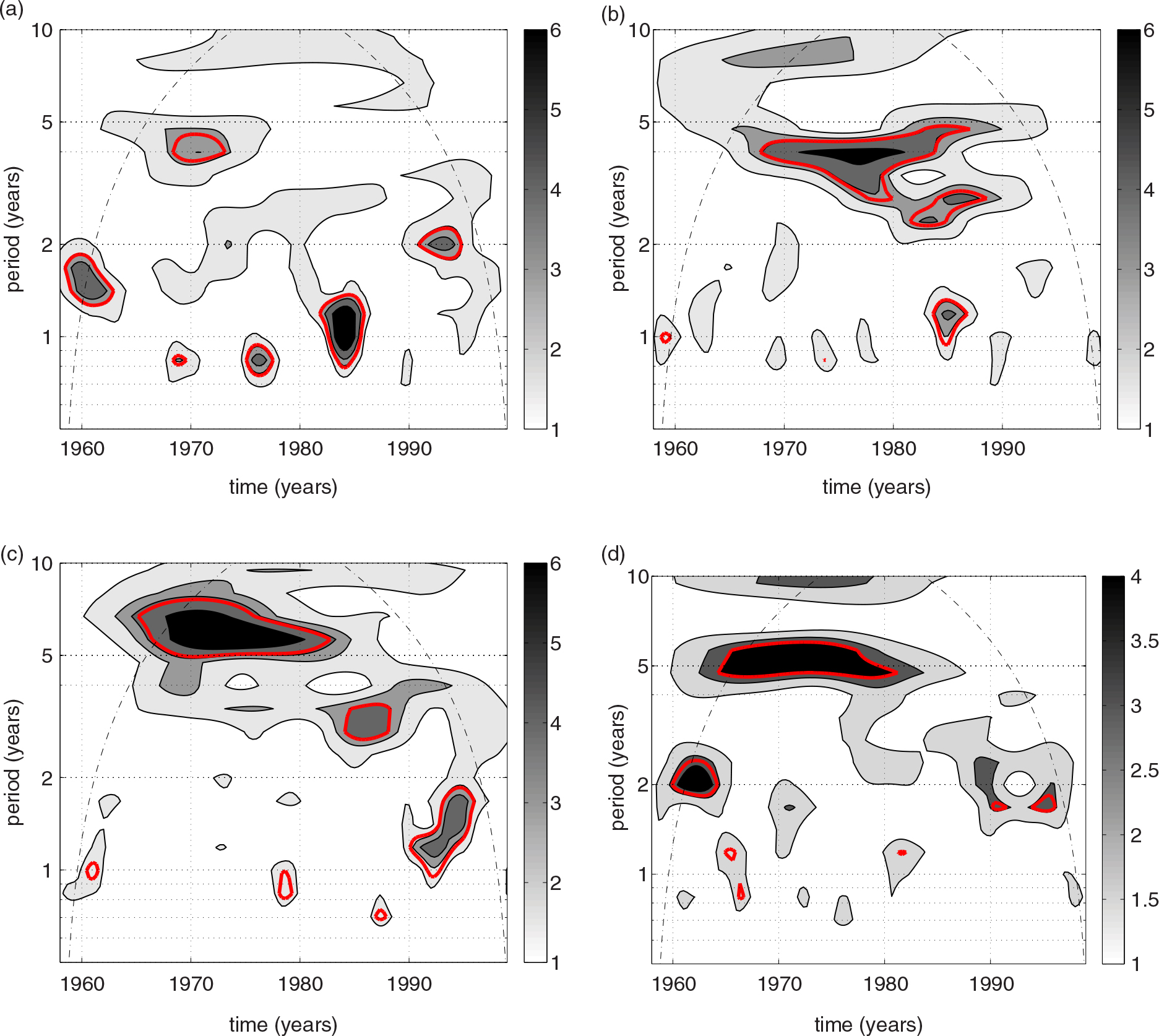
Fig. 11.
Global wavelet spectra of unfiltered and filtered NAO-index at Z 500. CMIP3 model runs and NCEP/NCAR and ERA40 re-analysis, DJF from 1958 to 1999. (a) unfiltered, (b) bandpass-filtered 7–15 yr. The wavelet transformation and filtering was performed with the Morlet wavelet.
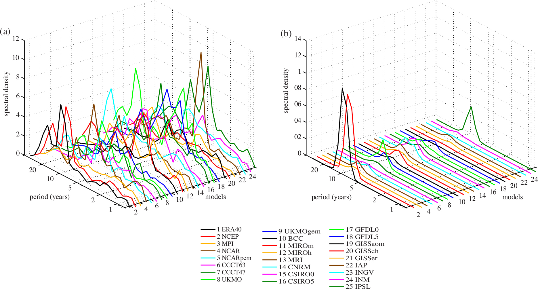
Fig. 12.
Global wavelet spectra of unfiltered and filtered PNA-index at Z 500. CMIP3 model runs and NCEP/ NCAR and ERA40 re-analysis, DJF from 1958 to 1999. (a) unfiltered, (b) bandpass-filtered 2–4 yr. The wavelet transformation and filtering was performed with the Morlet wavelet.
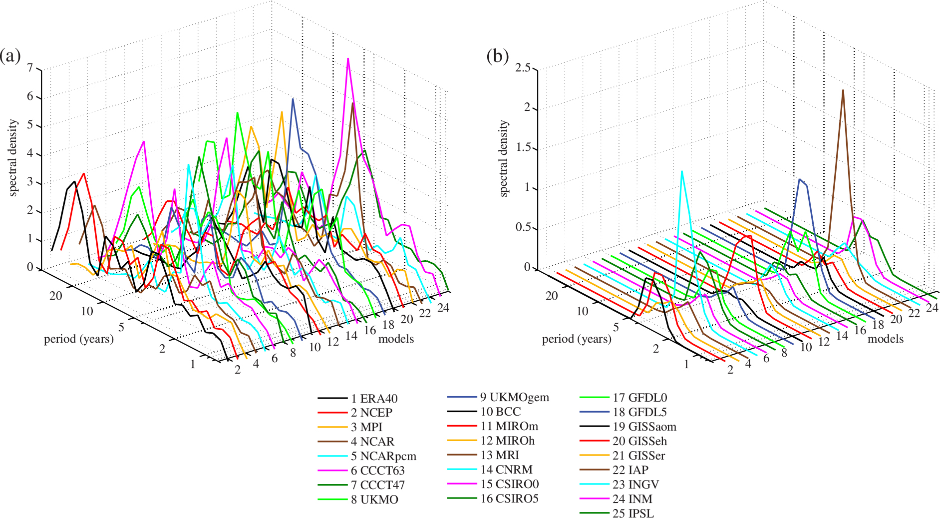
Fig. 13.
Global wavelet spectra of unfiltered and filtered PNA-index at Z 500. AMIP3 model runs and NCEP/NCAR and ERA40 re-analysis, DJF from 1979 to 1999. (a) unfiltered, (b) bandpass-filtered 2–4 yr. The wavelet transformation and filtering was performed with the Morlet wavelet.
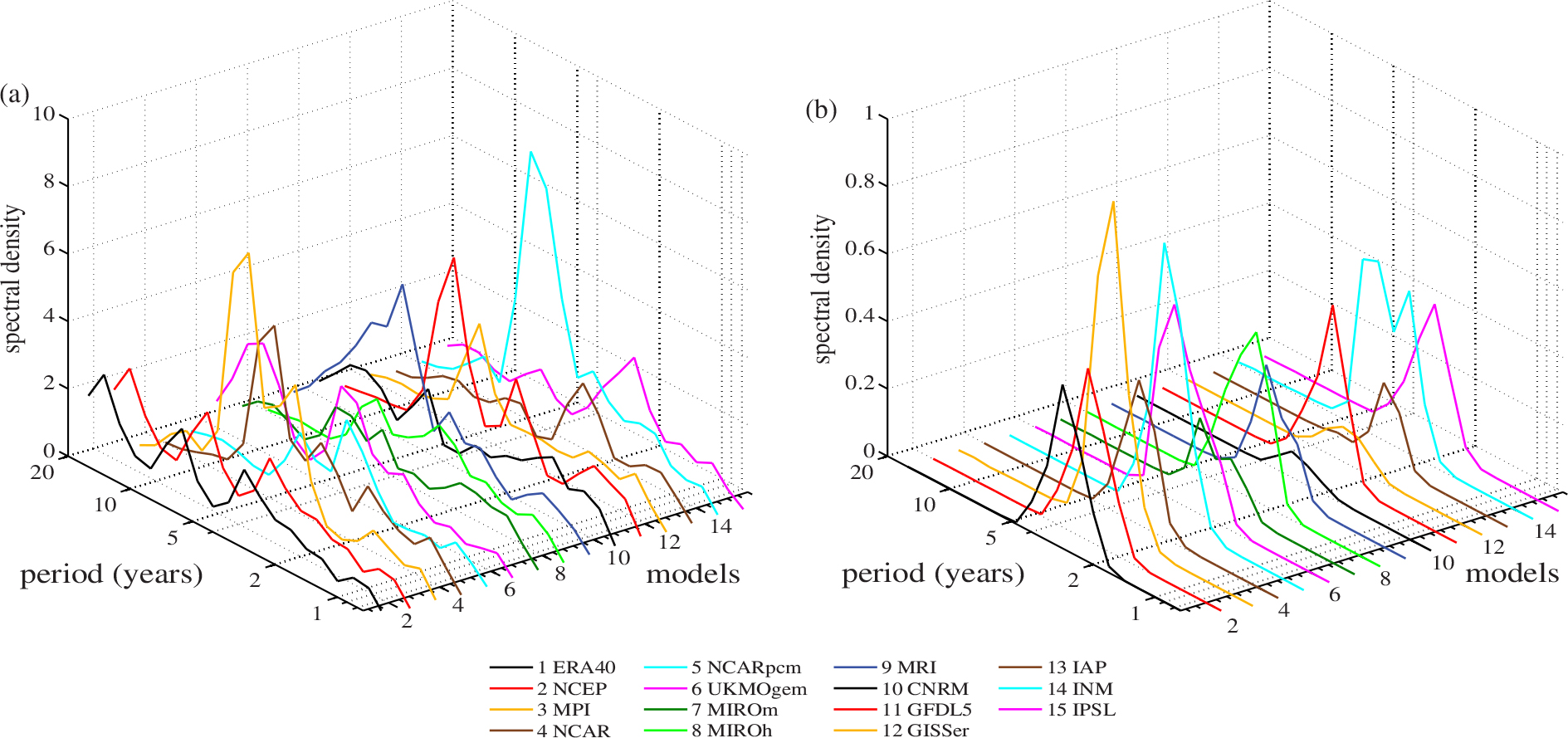
Fig. 14.
Summary of the NAO patterns and their relation to ATL-u-EOF1 for ERA40 re-analysis (a–d) and ECHAM5/MPI-OM (e–h). DJF-data from 1958 to 1999. From left to right: the NAO pattern (a, e); the regression pattern of the global geopotential height field at 500hPa onto ATL-u-PC1 at 250hPa (b, f); the regression pattern of the global zonal wind field at 250hPa onto ATL-u-PC1 at 250hPa (colours with overlaid Atlantic mean jet) (c, g); the vertical profile of explained variance between the NAO-index and the sectoral ATL-u-PC1 at each height (d, h).
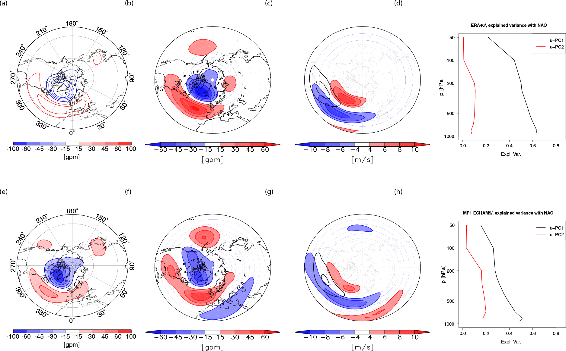
Fig. 15.
Summary of the EA patterns and their relation to ATL-u-EOF2 for ERA40 re-analysis (a–d) and ECHAM5/MPI-OM (e–h). DJF-data from 1958 to 1999. From left to right: the EA pattern (a, e); the regression pattern of the global geopotential height field at 500hPa onto ATL-u-PC2 at 250hPa (b, f); the regression pattern of the global zonal wind field at 250hPa onto ATL-u-PC2 at 250hPa (colours with overlaid Atlantic mean jet) (c, g); the vertical profile of explained variance between the EA-index and the sectoral ATL-u-PC2 at each height (d, h).
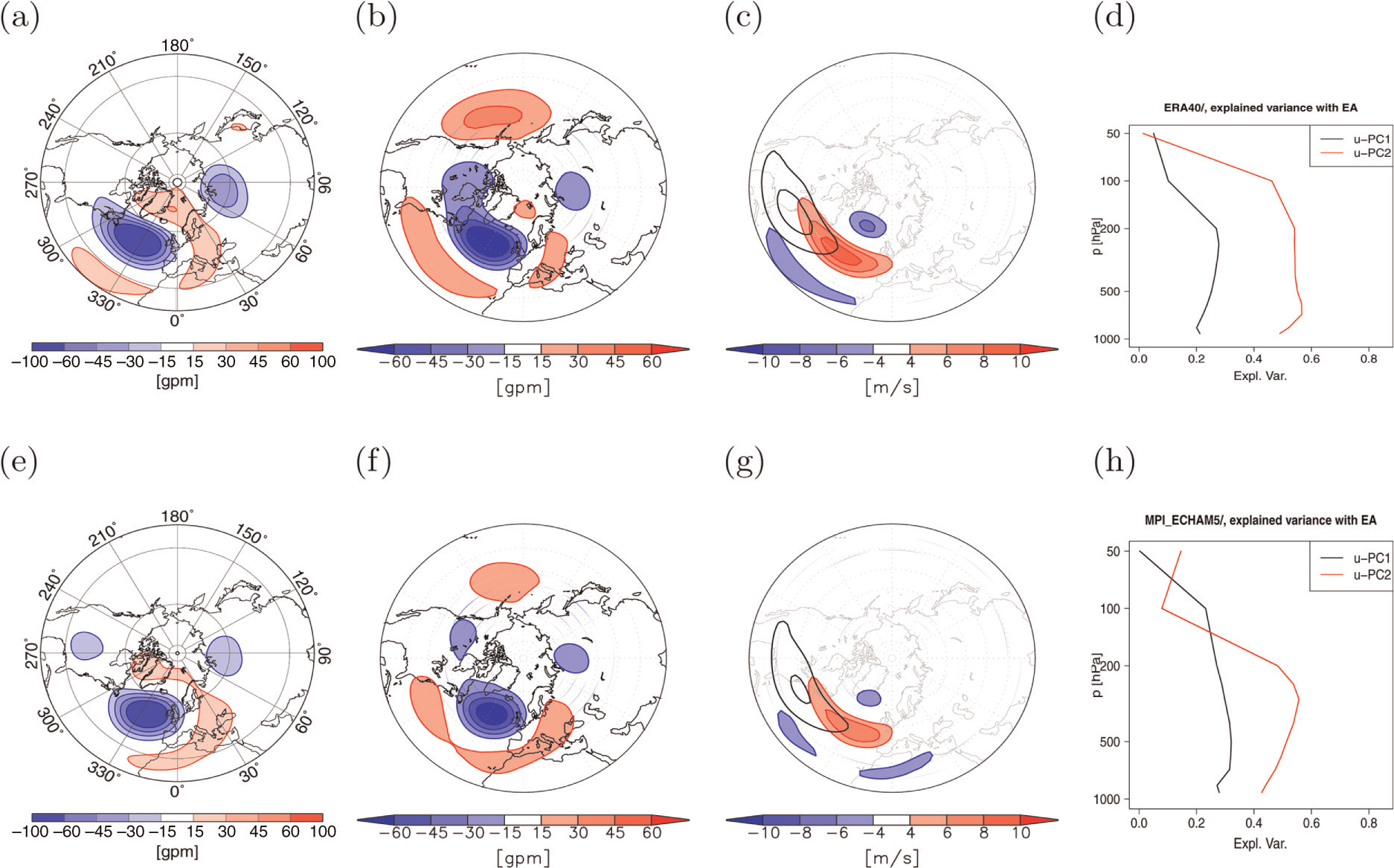
Fig. 16.
Summary of the PNA patterns and their relation to PAC-u-EOF1 for ERA40 re-analysis (a–d) and UKMO HadGEM1 (e–h). DJF-data from 1958 to 1999. From left to right: the PNA pattern (a, e); the regression pattern of the global geopotential height field at 500hPa onto PAC-u-PC1 at 250hPa (b, f); the regression pattern of the global zonal wind field at 250hPa onto PAC-u-PC1 at 250hPa (colours with overlaid Pacific mean jet) (c, g); the vertical profile of explained variance between the PNA-index and the sectoral PAC-u-PC1 at each height (d, h).
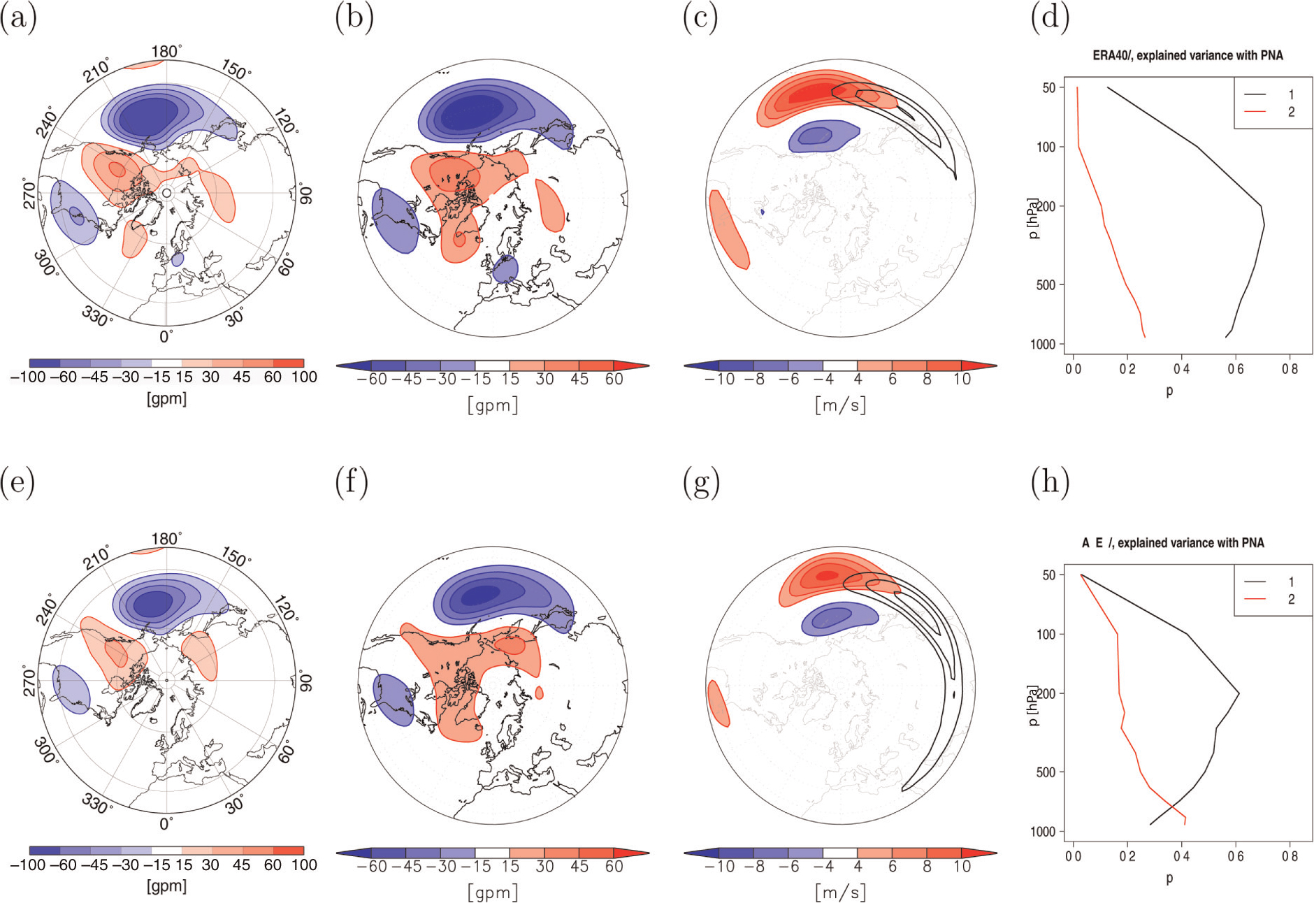
Fig. 17.
Summary of the WP patterns and their relation to PAC-u-EOF2 for ERA40 re-analysis (a–d) and UKMO HadGEM1 (e–h). DJF-data from 1958 to 1999. From left to right: the WP pattern (a, e); the regression pattern of the global geopotential height field at 500hPa onto PAC-u-PC2 at 250hPa (b, f); the regression pattern of the global zonal wind field at 250hPa onto PAC-u-PC2 at 250hPa (colours with overlaid Pacific mean jet) (c, g); the vertical profile of explained variance between the WP-index and the sectoral PAC-u-PC2 at each height (d, h).
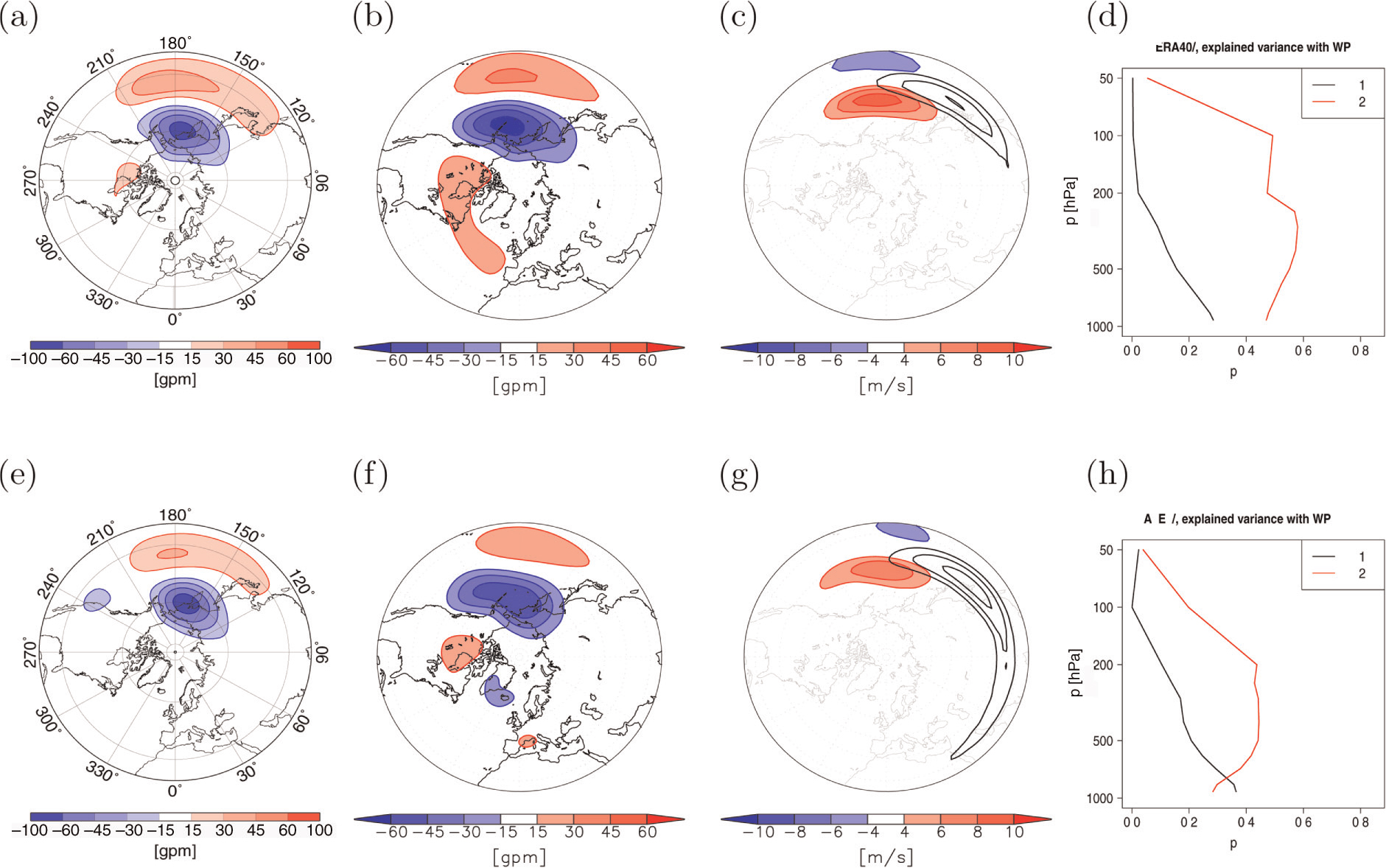
Fig. 18.
Performance metrics for NAO (a) and EA (b) and their relations to ATL-u-EOFs. The columns of the metric give from left to right the values of the skill scores for teleconnection patterns, ATL-u-EOFs at 250hPa, regression patterns of the geopotential height field at 500hPa onto ATL-u-PC at 250hPa, comparison of teleconnection pattern and regression pattern of the same model. Models are sorted according to the skill score of the NAO and EA patterns, respectively.
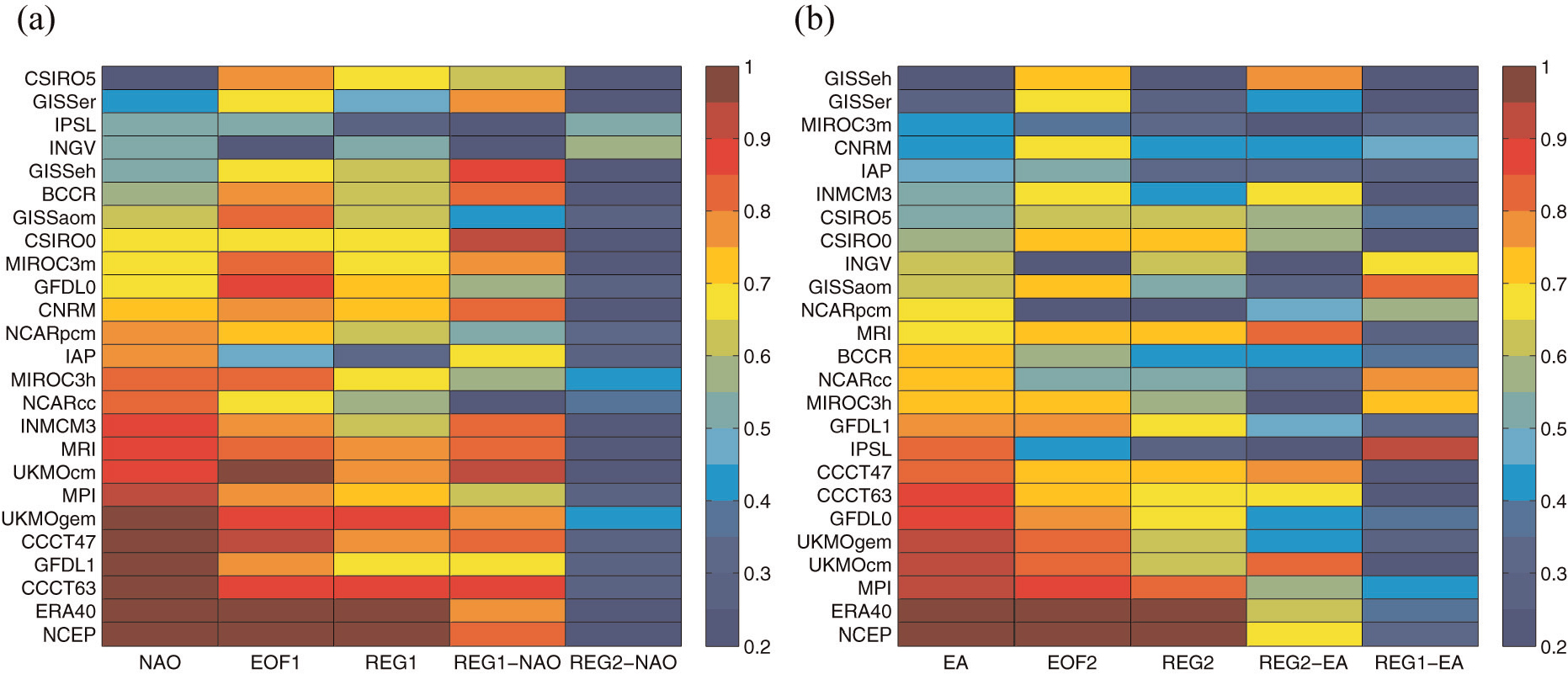
Fig. 19.
Same as in Fig. 18, but for PNA (a) and WP (b) and their relations to PAC-u-EOFs. Models are sorted according to the skill score of the PNA and WP patterns, respectively.

Fig. 20.
Left: Performance metrics as in Fig. 18, but for those model showing same relationship between teleconnection and zonal wind variability as the re-analysis. Models are sorted according to the skill score of the NAO (a) and EA (c) patterns, respectively. (b, d) Vertical profiles of shared variance with the related ATL-u-PCs for the selected models.
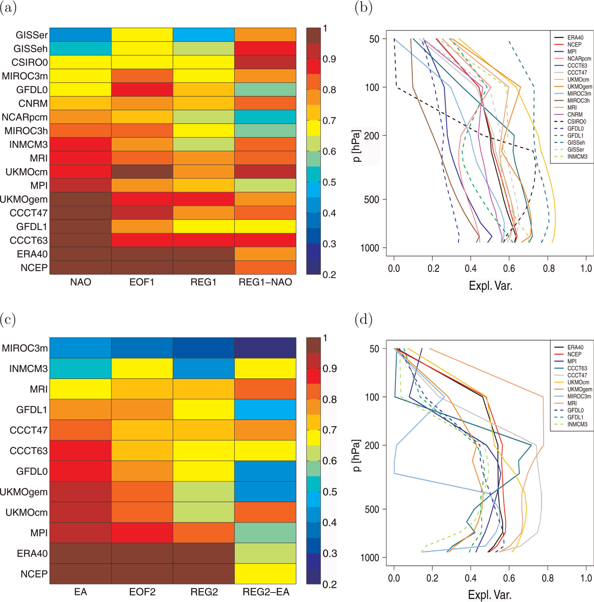
Fig. 21.
Same as in Fig. 20 but for the PNA (a, b) and WP (c, d) patterns and their relation to PAC-u-EOFs. Models are sorted according to the skill score of the PNA and WP patterns, respectively.
