Fig. 1.
Time series of 1979–2010 September SIC index (defined for region of highest variance, 70°–85°N, 90°–210°E), showing both the ‘observed’ index [(a) the grey lines show the time series mean and ±0.5 SD), and the detrended, standardised sea ice index for the same time period (b). The bottom panel (c) shows the detrended and standardised SIC index for 1950–2010 for comparison. Selected years from the highest SIC (+0.5 SD for satellite period, top 10 yr for the long time series) subset are indicated by the red squares on the time series, and the subset belonging to the lowest years (−0.5 SD for satellite period, lowest 10 yr for the long time series) are indicated by blue triangles.
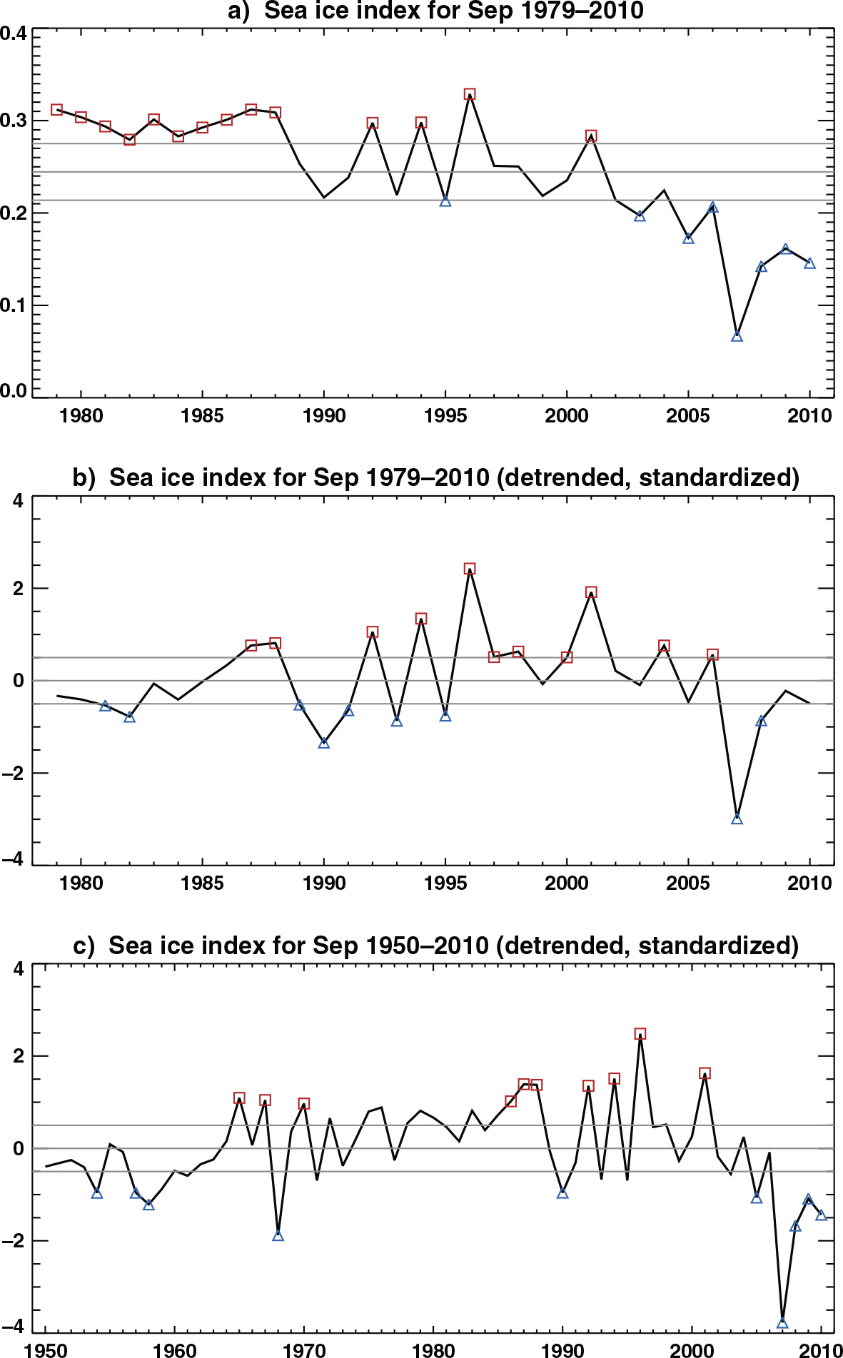
Fig. 2.
Comparison of Eurasian sea ice index shown in Fig. 1 with four additional sea ice indexes, as derived for different regions for 1950–2010. The regions and their selected boundaries are: Arctic Ocean (ArcO, 70°–85°N, 0°–360°W), Barents/Kara Sea (BarKar, 70°–85°N, 30°–90°E), Chuckchi Sea (Chuck, 70°–85°N, 180°–157°W) and Eurasia and Barents/Kara Sea (EKB, 70°–85°N, 30°–210°E).
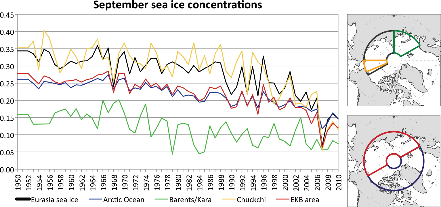
Fig. 3.
September SIC difference between lowest and highest (±0.5 SD) sea ice index years. The difference of the original data for 1979–2009 is shown in the top left panel (a), the difference of the composite for the detrended data for the same period is shown in (b) (middle panel). The difference of the detrended data for 1950–2009 is shown in (c) (bottom left panel) for comparison. Statistically significant regions are hatched (95% significance: back hash and 99% significance: forward hash). The variance for September sea ice from the original data for the two time periods is shown in (d) (1979–2009) and (e) (1950–2009). The box used to derive the sea ice index is outlined in (d).
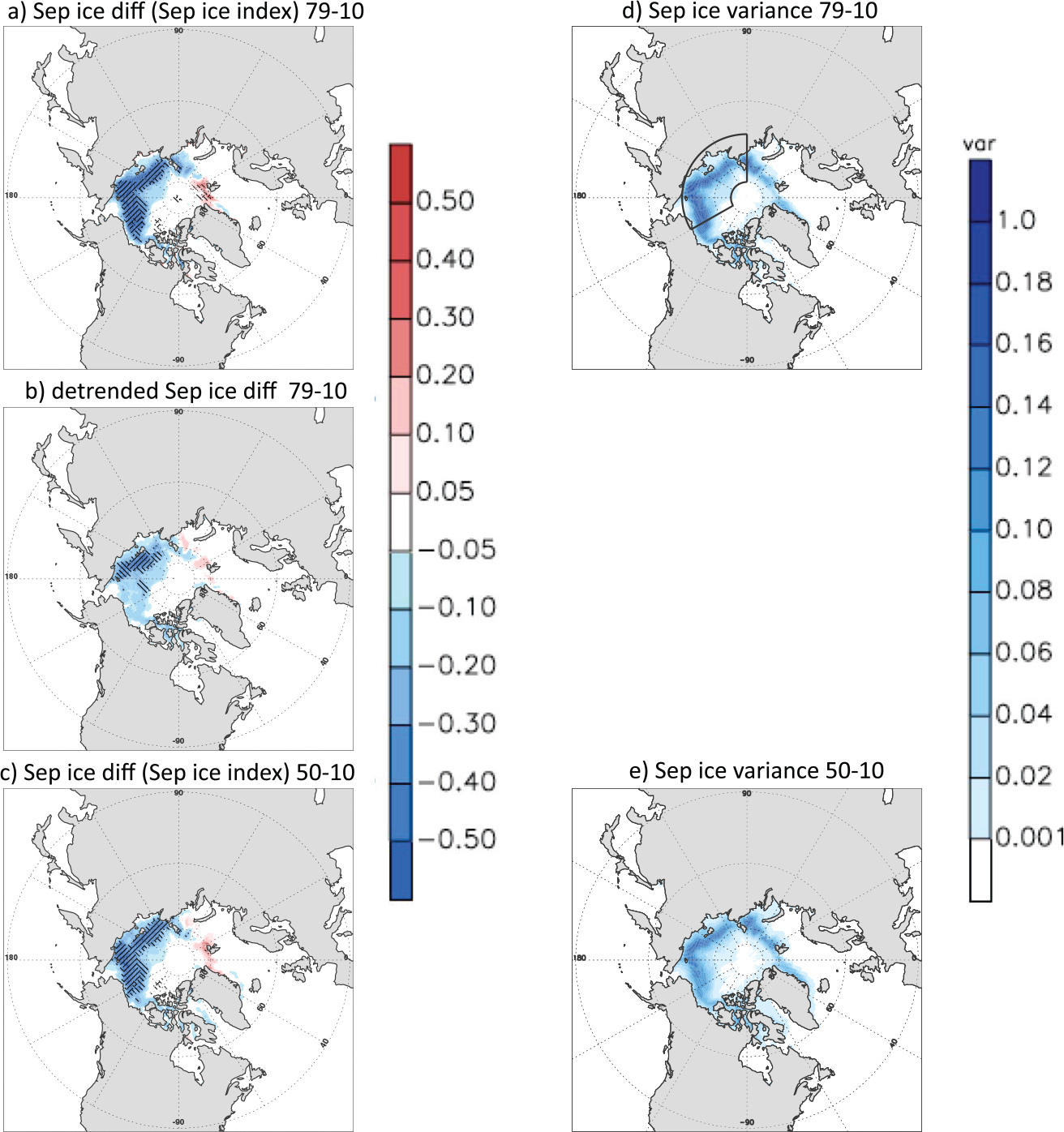
Fig. 4.
Illustration of how composite differences are generated. (a) The composite of geopotential height at 500 hPa using the selected low SIC years; the composites for the high SIC years are shown in (b). The difference between panel a and panel b is shown in the panel c and highlights the main features that differentiate the two conditions from each other. (d) to (f) are same as (a) to (c) but for 1950–2010.
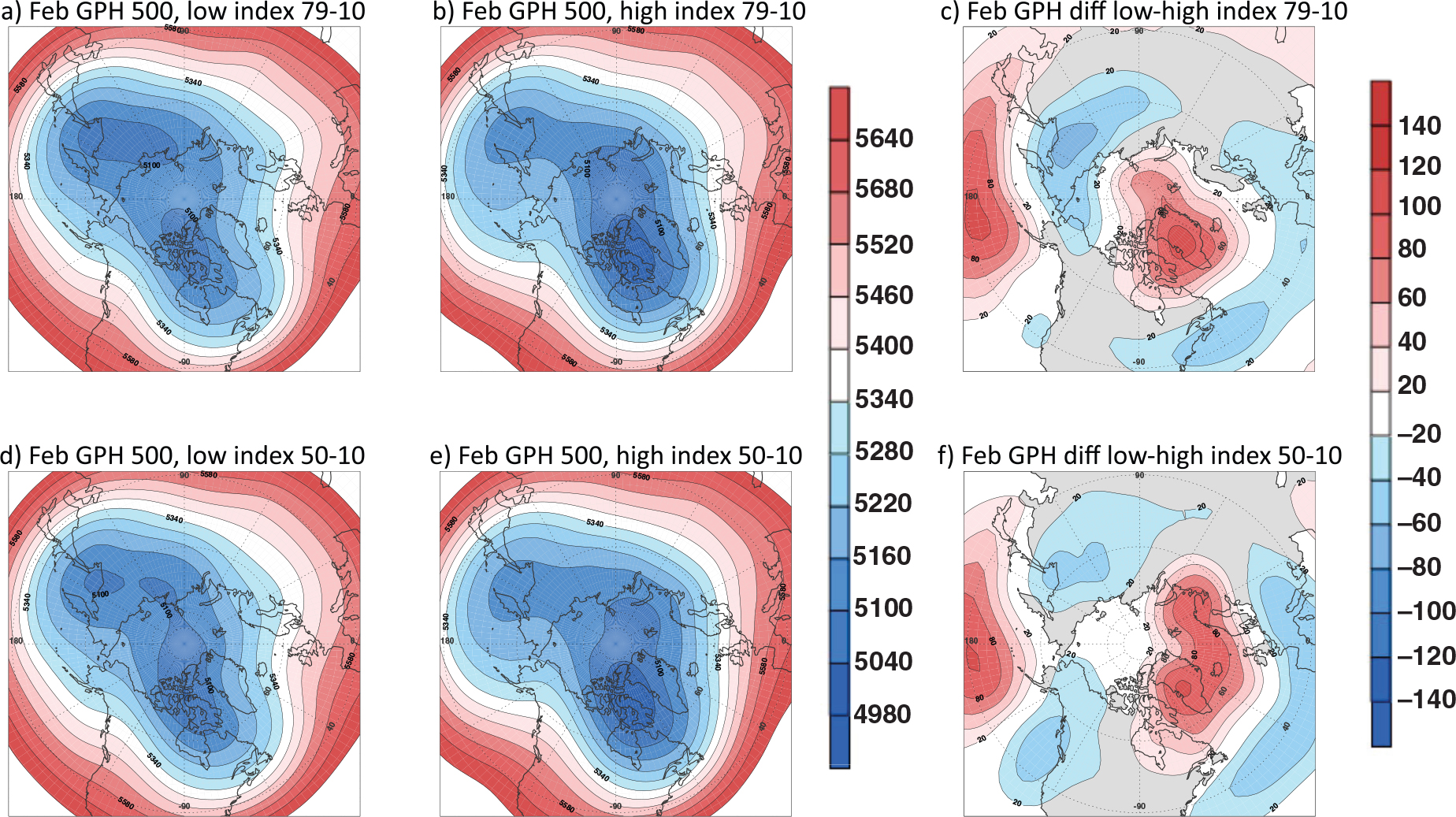
Table 1. Correlation coefficients between the various regions’ SIC indexes for both the satellite period (1979–2010) and long period (1950–2010) time series
[i] Statistical significance at the 95% levels is shown in italics.
Fig. 5.
Difference between lowest and highest (±0.5 SD) years from 1979 to 2010 using September SIC index for region 70°–85°N, 90°–210°E of T1000 (temperature at 1000 hPa, shaded) for September, October, November (top to bottom) of NNR original data (left panels, a–c) and detrended NNR data (middle panels, d–f), and for detrended NNR data from the longer time period (1950–2010) in rightmost panels (g–i). Statistically significant areas are enclosed in black contours at the 95 and 99% significance level.
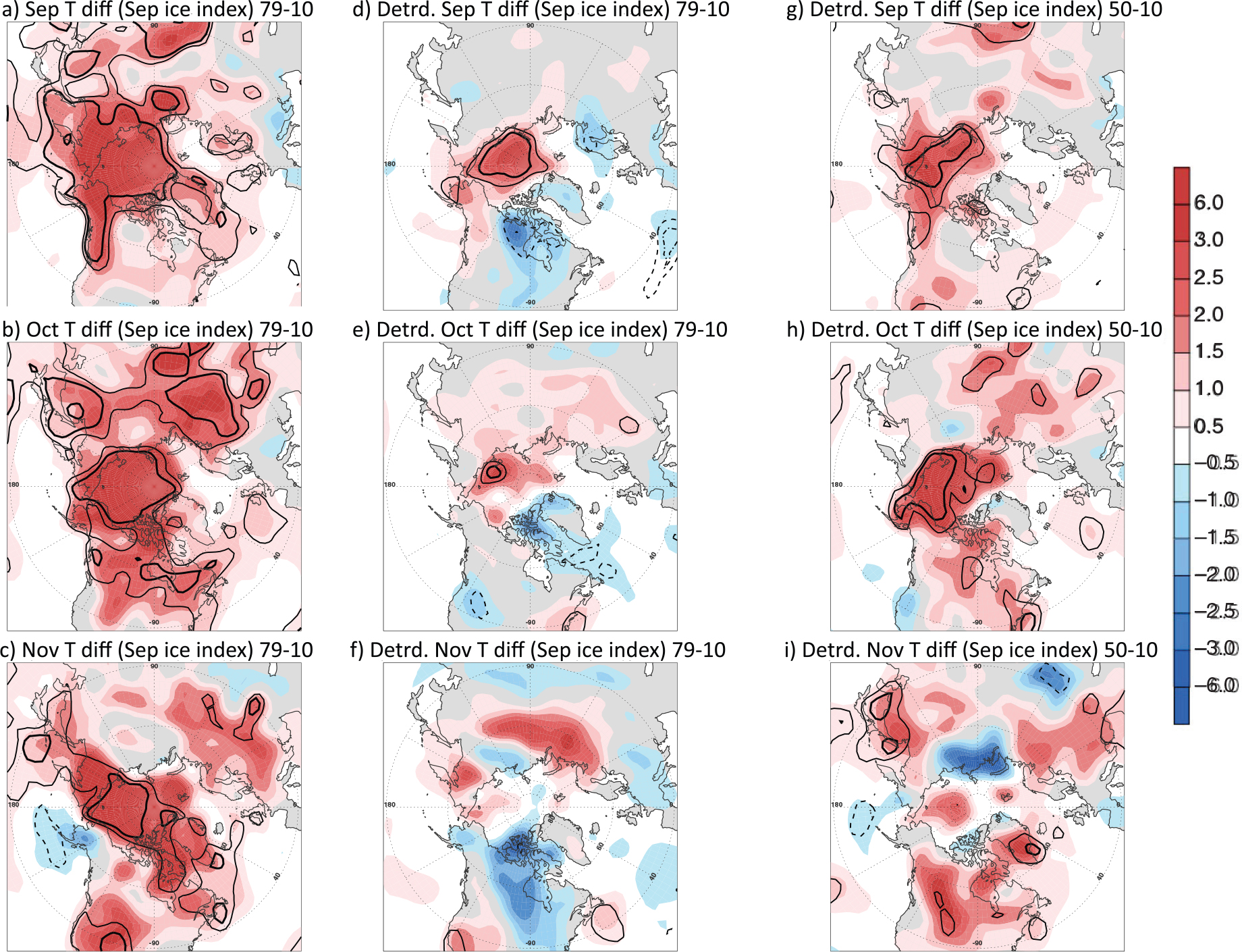
Fig. 6.
Same as Fig. 5 but for difference between lowest and highest (±0.5 SD) years from 1979 to 2010 using September SIC index for December, January, February (top to bottom) of NNR original data (left panels, a–c) and detrended NNR data (middle panels, d–f), and for detrended NNR data from the longer time period (1950–2010) in rightmost panels (g–i).
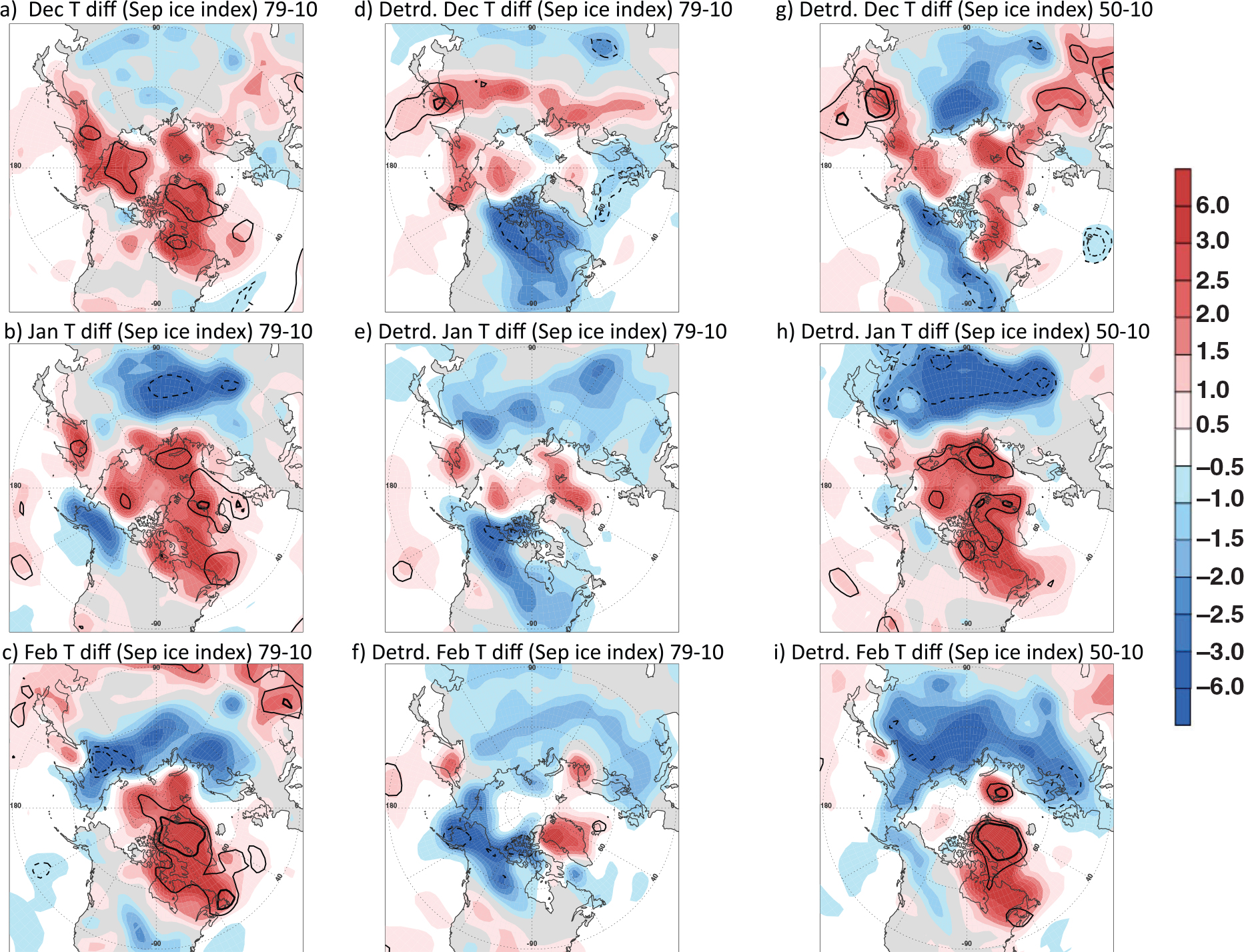
Fig. 7.
Same as Fig. 5 but for geopotential height at 500 hPa (GPH 500 hPa) for September, October, November (top to bottom) of NNR original data (left panels, a–c), detrended NNR data (middle panels, d–f) and for detrended NNR data from the longer time period (1950–2010) in rightmost panels (g–i).
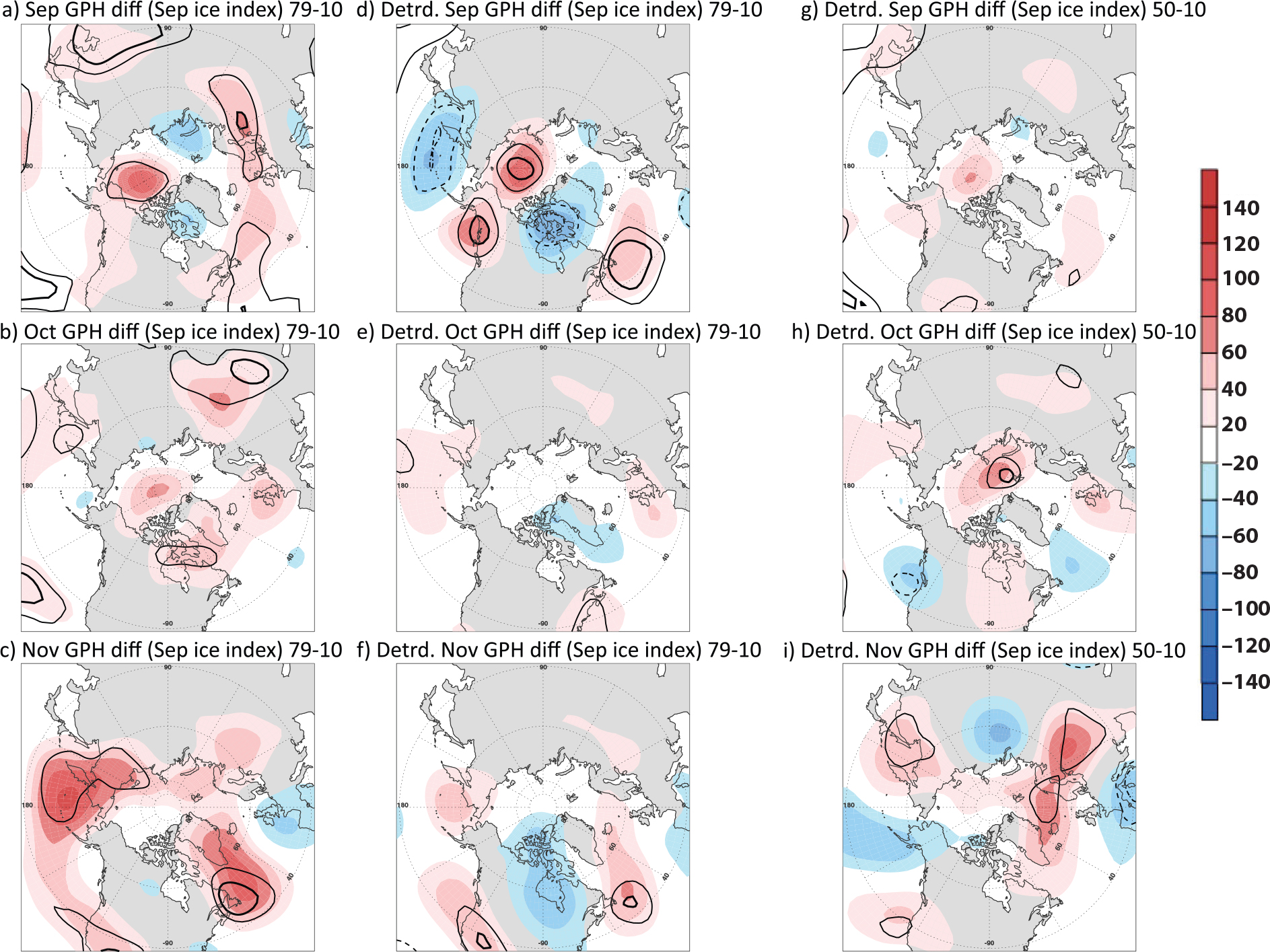
Fig. 8.
Same as Fig. 7 but for geopotential height at 500 hPa (GPH 500 hPa) for December, January, February (top to bottom) of NNR original data (left panels, a–c), detrended NNR data (middle panels, d–f) and for detrended NNR data from the longer time period (1950–2010) in rightmost panels (g–i).
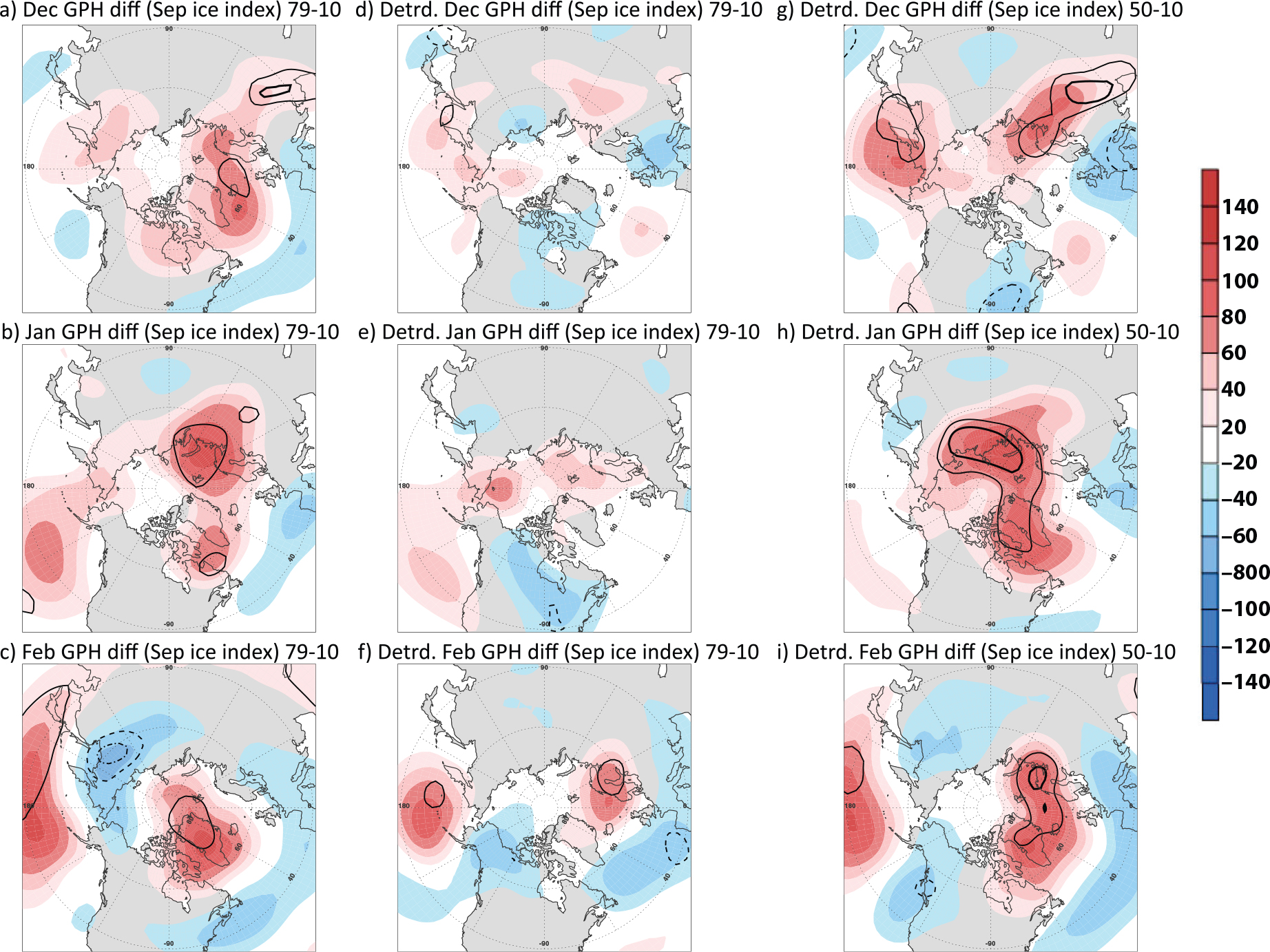
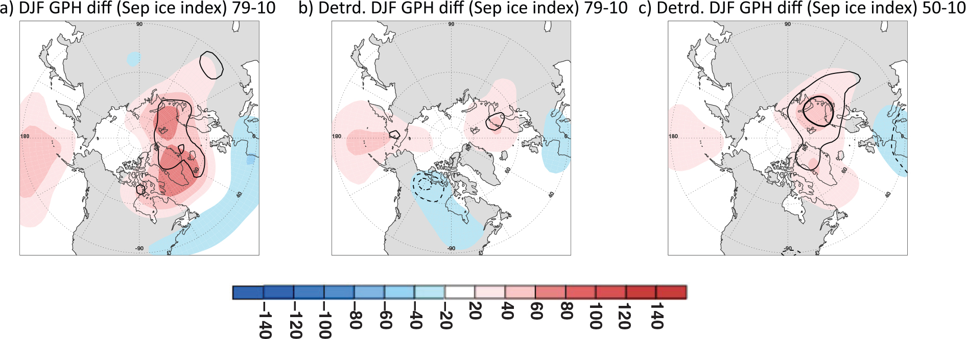
Fig. 9.
Same as Fig. 8 but for geopotential height at 500 hPa, for the winter mean (December–February, DJF) of NNR original data (a), detrended NNR data (b) and for detrended NNR data from the longer time period (1950–2010, c).