Fig. 1.
Normalised monthly mean time series of (a) the leading phase, (b) real and (c) imaginary parts of the leading complex principal component, and three time series are obtained from deviations from their means divided by their SDs from 1979 to 2010 (for a total of 384 months).
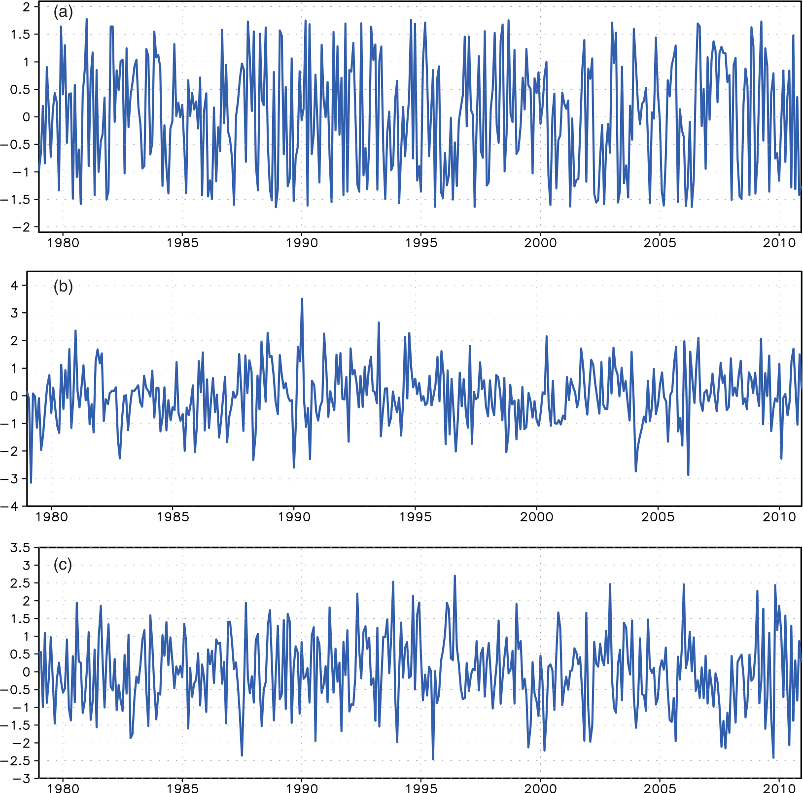
Table 1. Frequencies for different phase ranges in the summer months (July to September) from 1979 to 2010
Fig. 2.
(a) Composite of summer monthly mean surface wind anomalies for the ‘0°’(θ < 45° or θ≥315°) phase of the leading surface wind pattern, (b)–(d) as in (a) but for the ‘90°’(135° > θ≥45°), ‘180°’(225° > θ≥135°), ‘270°’(315° > θ≥225°) phases, respectively; (e)–(h) as in (a)–(d) but for corresponding SLP anomalies; units: m s−1 in (a)–(d); hPa in (e)–(h).
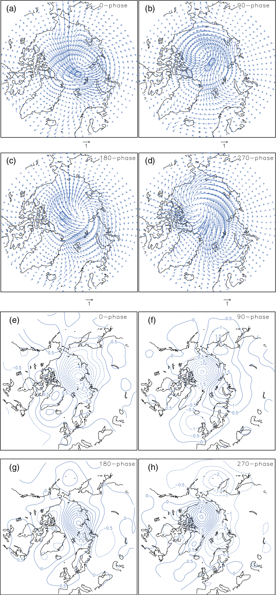
Fig. 3.
As in Fig. 2, but for the second wind pattern.
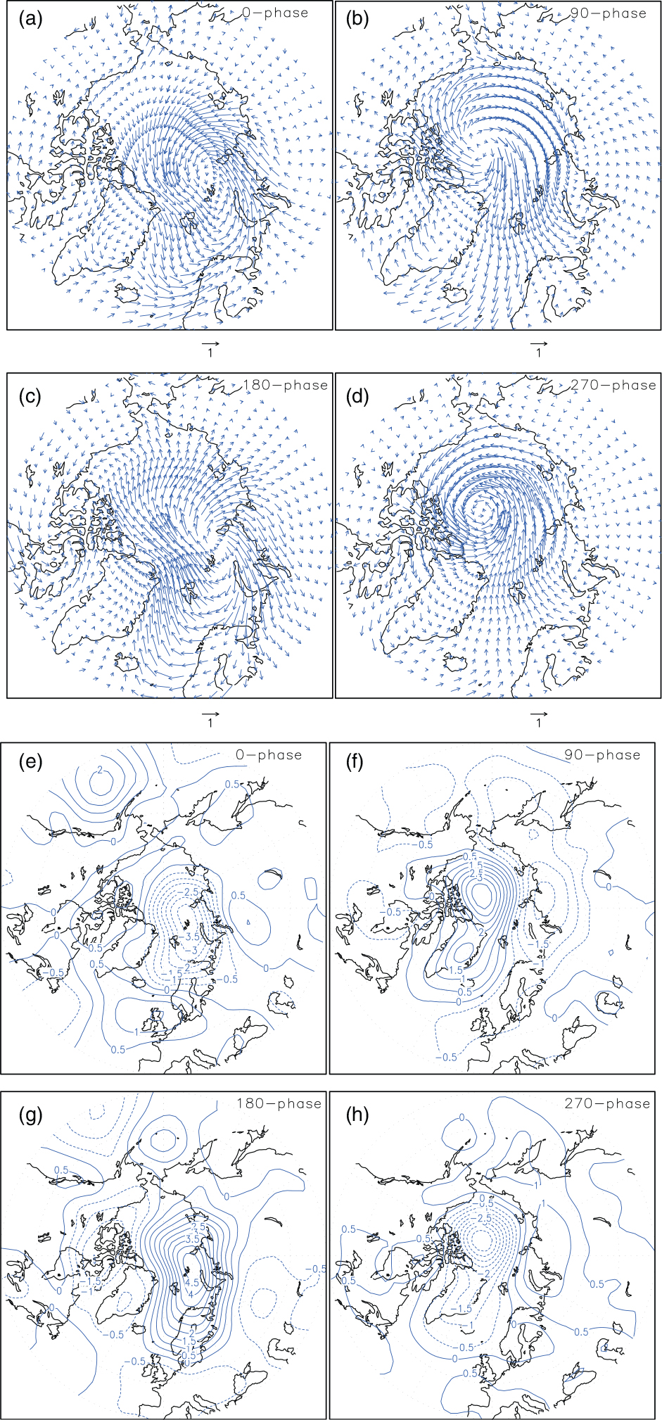
Fig. 4.
(a) Composite of summer monthly mean 500 hPa height anomalies for the ‘0°’(θ < 45° or θ≥315°) phase of the leading wind pattern, (b)–(d) as in (a) but for the ‘90°’(135° > θ≥45°), ‘180°’(225° > θ≥135°), ‘270°’(315° > θ≥225°) phases, respectively; (e) composite of summer monthly mean 500 hPa heights for the ‘0°’ (green contour) and ‘180°’ (red contour) phases, (f) same as in (e), but for the ‘90°’ (green contour) and ‘270°’ (red contour) phases, (g) and (h), respectively, same as in (e) and (f), but for the second wind pattern, contour intervals are 10 in (a)–(d) and 25 gpm in (e)–(h), respectively.
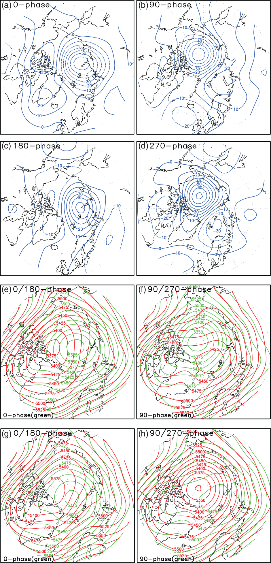
Fig. 5.
Normalised time series of (a) the NLS and (b) AD patterns, respectively, derived from summer (July to September) means of the real and imaginary parts of the leading complex principal component, (c) and (d), respectively, as in (a) and (b), but for the NKS and CA patterns, derived from the second complex principal component, (e) normalised time series of Arctic September SIE (SIC > 15%), derived from BADC SIC data, red-dashed lines represent their trends, five time series are obtained from deviations from their means divided by their SDs.
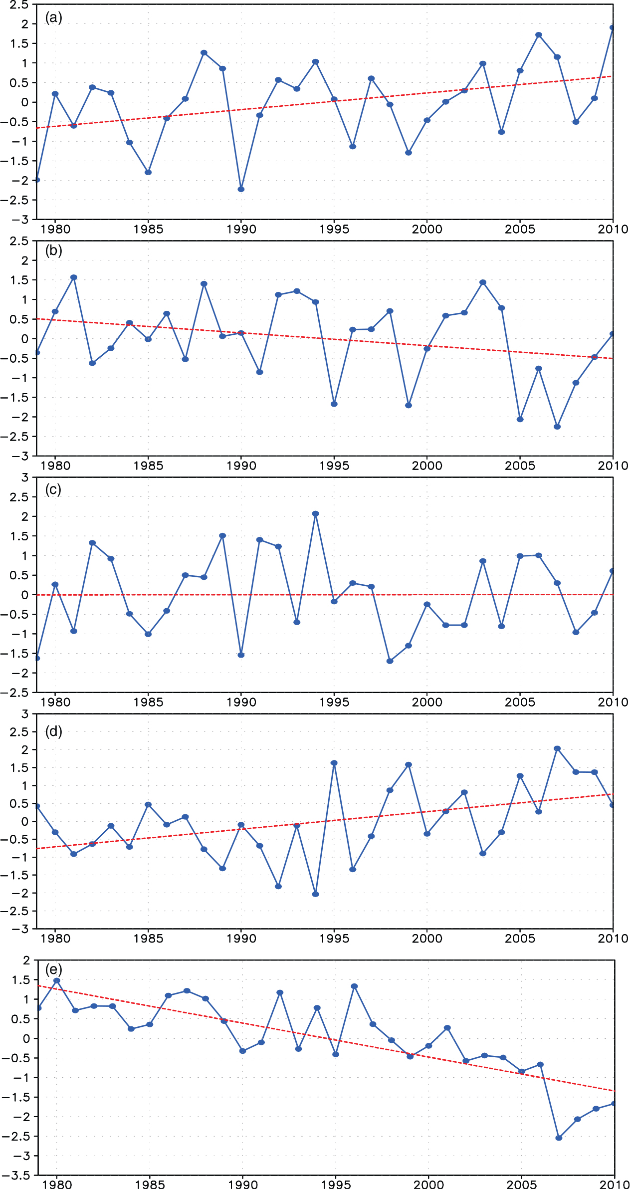
Fig. 6.
Summer (July to September) mean surface wind anomalies in (a) 1995, (b) 1999, (c) 2005, (d) 2007, (e)–(h) as in (a)–(d), respectively, but for summer mean SLP anomalies; units: m s−1 in (a)–(d) and hPa in (e)–(h).
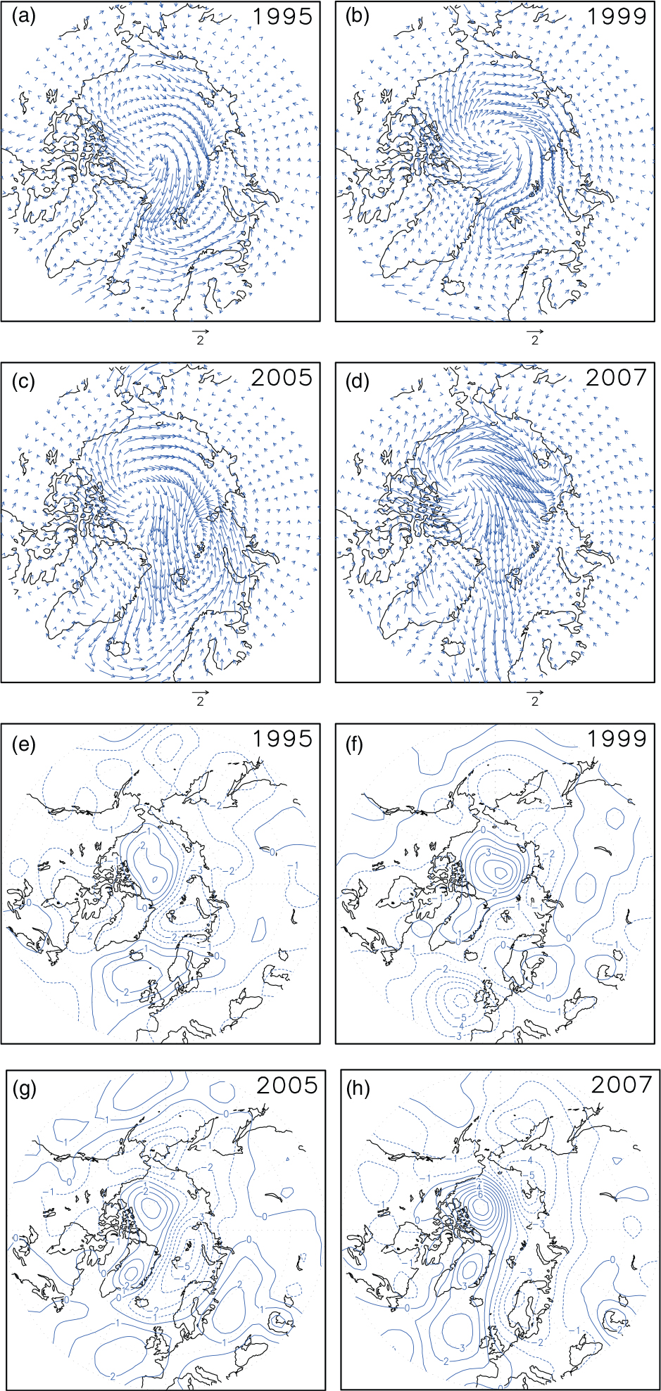
Fig. 7.
(a) Frequencies of the negative phase of the AD pattern from July to September, (b) as in (a), but for the positive phase of the CA pattern, (c) cumulative frequencies of the positive phase of the CA pattern in the melting season from April to September.
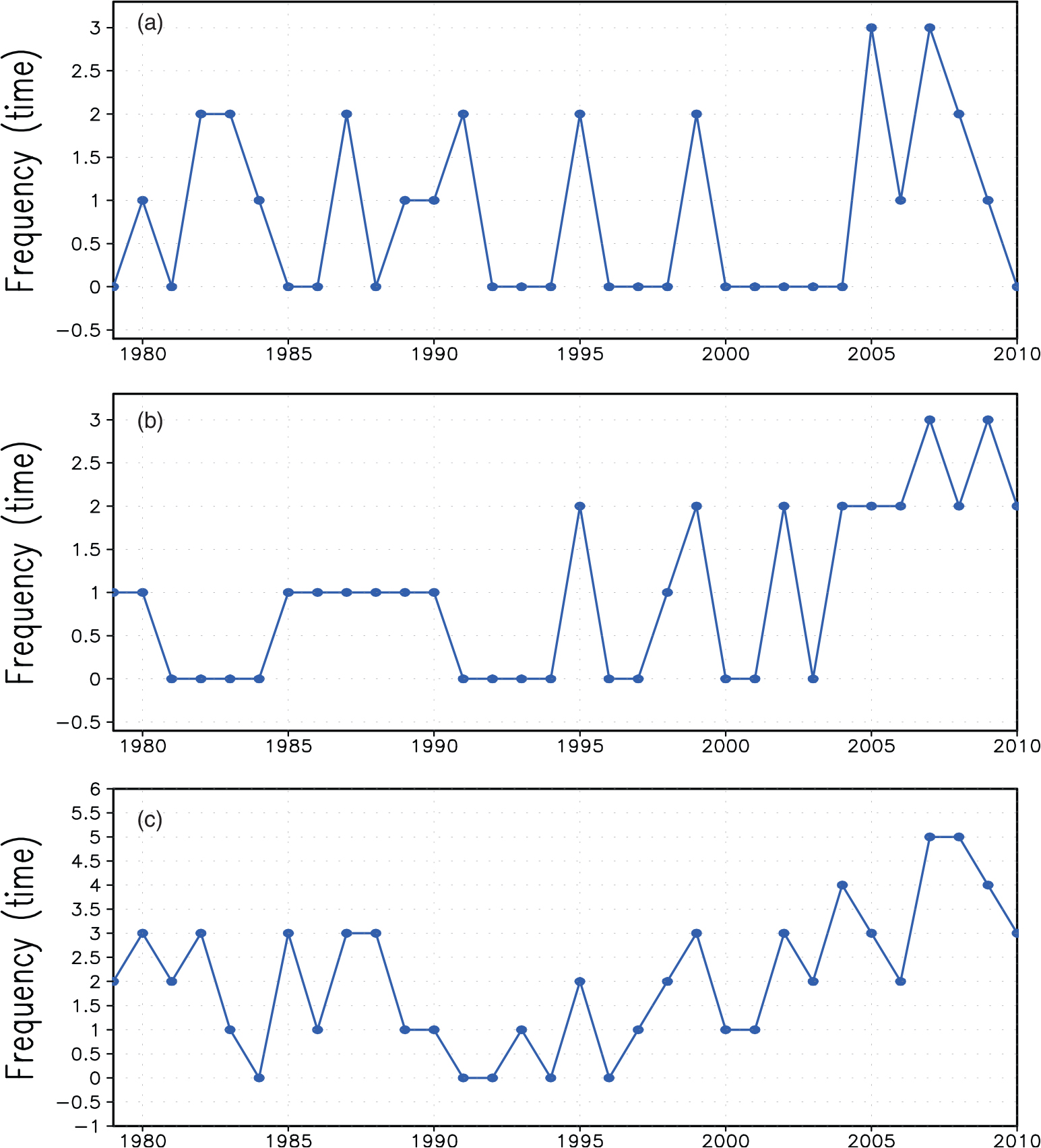
Fig. 8.
(a) September SIC anomalies derived from a linear regression on the converted normalised time series of the AD pattern, (b) as in (a) but for regressed on the normalised time series of the CA pattern, (c) as in (b) but for regressed on the trend in the CA pattern, (d) as in (c) but for regressed on the detrended time series of the CA pattern, colour-shading areas denote SIC anomalies exceeding the 95 and 99% significance levels, respectively.
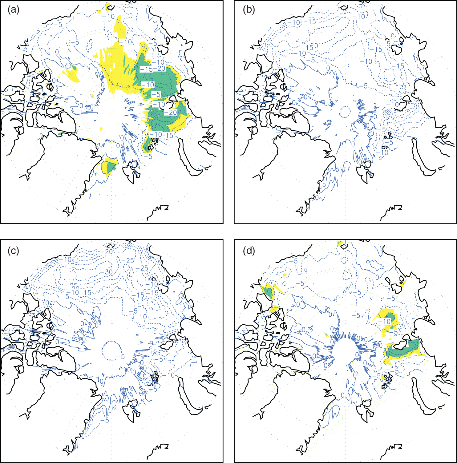
Fig. 9.
(a) Normalised time series of the AD pattern (blue line) and EOF3 (red line), their correlation is 0.91, both time series are obtained from deviations from their means divided by their SDs, (b) and (c) regression maps of summer mean SLP, regressed on the AD pattern and EOF3, respectively, colour-shading areas denote SLP anomalies exceeding the 95 and 99% significance levels, respectively.
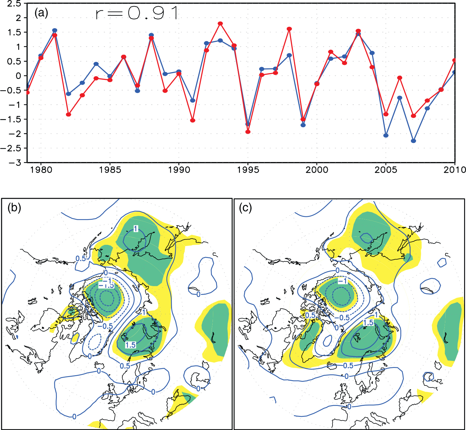
Fig. 10.
(a) Normalised time series of the CA pattern (blue line) and EOF2 (red line), their correlation is 0.52 (the correlation becomes 0.36 after removing their trends), both time series are obtained from deviations from their means divided by their SDs, (b) and (c) regression maps of summer mean SLP, regressed on the CA pattern and EOF2, respectively, (d) and (e) as in (b) and (c), respectively, but for regressed on their detrended time series, colour-shading areas denote SLP anomalies exceeding the 95 and 99% significance levels, respectively.
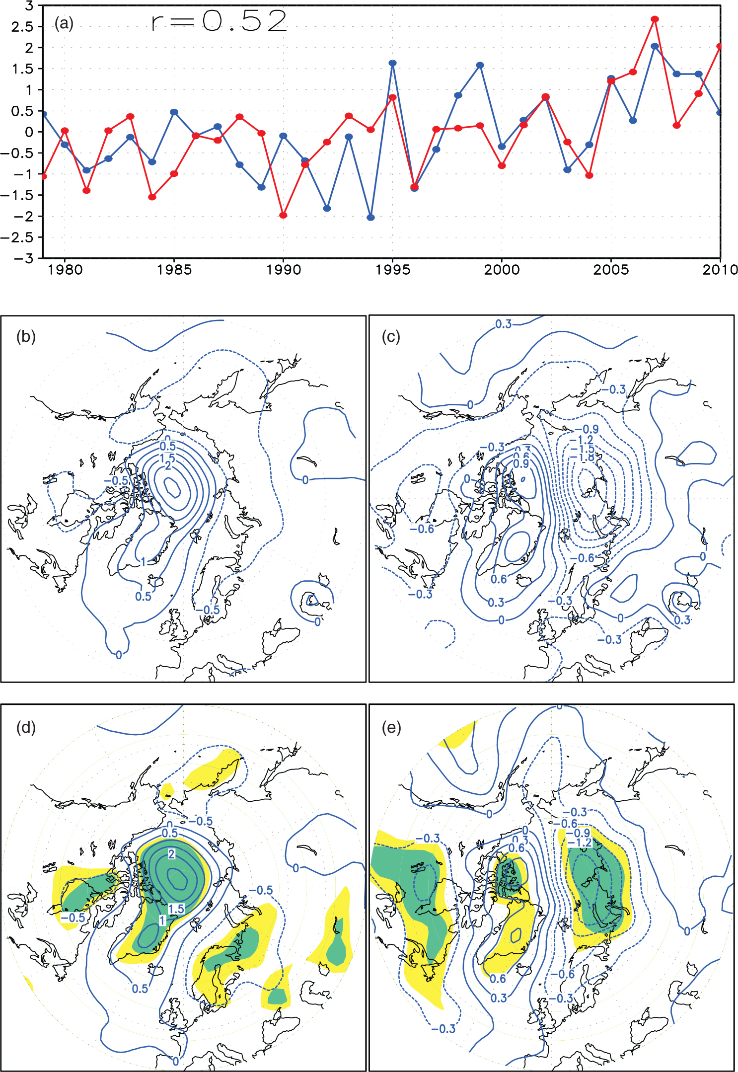
Fig. 11.
(a) Five-year running means of the normalised time series of the CA pattern, (b) as in (a) but for spring (April to June) mean, two normalised time series are obtained from deviations from their means divided by their SDs.