Fig. 1.
The truth initial height and wind fields. (a) Case I and observation networks and (b) Case II. The grey solid square in (a) denotes the observation site of OBSN I (x=25.3, y=15.7), the grey diamonds show the observation sites of OBSN II (y=15) and the grey circles indicate the observation sites of OBSN III (x=15). The OBSN IV includes both the grey diamonds (OBSN II) and grey circles (OBSN III).
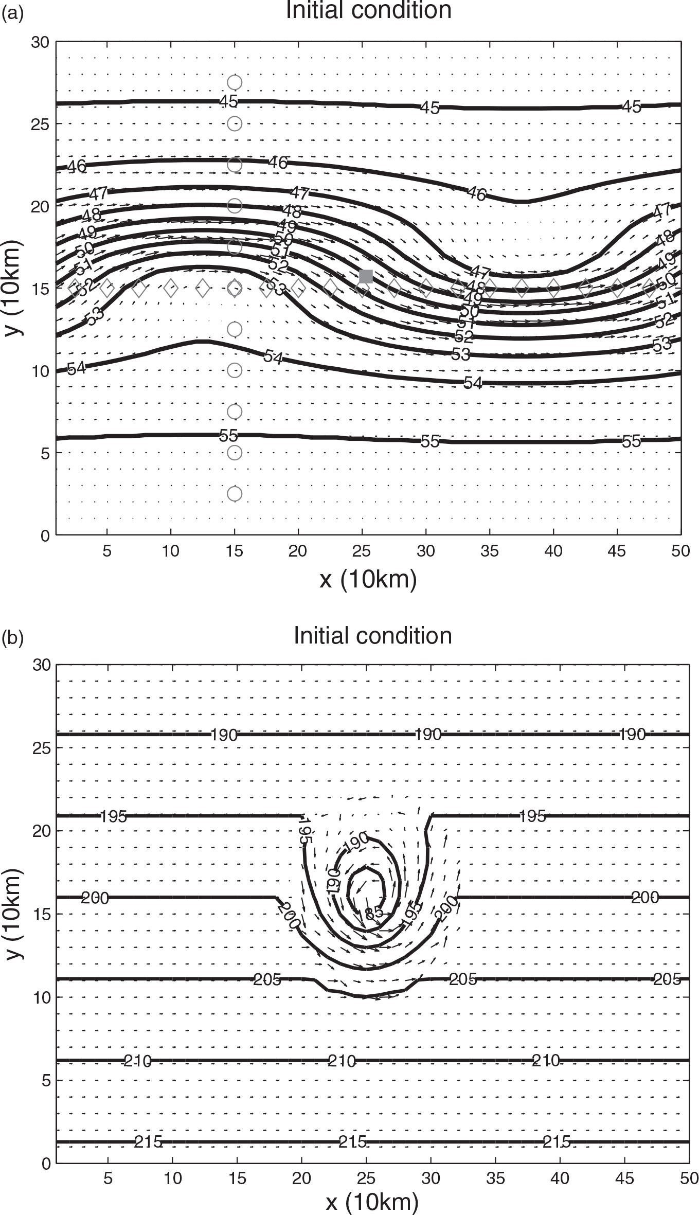
Table 1. Experimental design
Fig. 2.
The normalised RMS error of Case I for Experiments CTRL (thin light grey solid line), Nudging (thick light grey solid line), EnKF (dark grey solid line), HNEnKF (black dash-dotted line) and EnKS (dark grey dash-dotted line). The baseline configuration (OBSF 3 and OBSN II) is used for all of the data assimilation experiments. (a) Height field and (b) wind field.
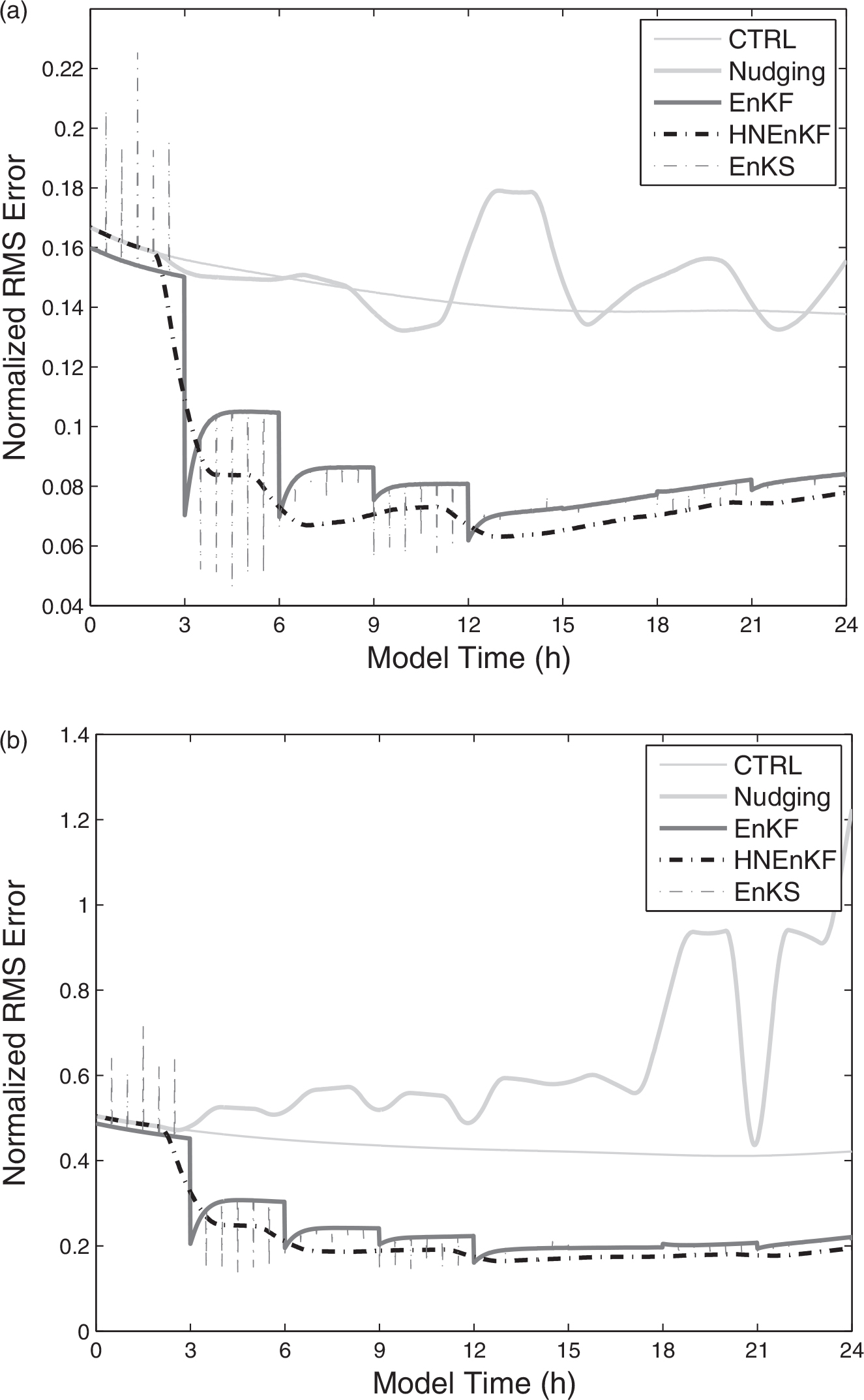
Fig. 3.
Same as Fig. 2, except for Case II.
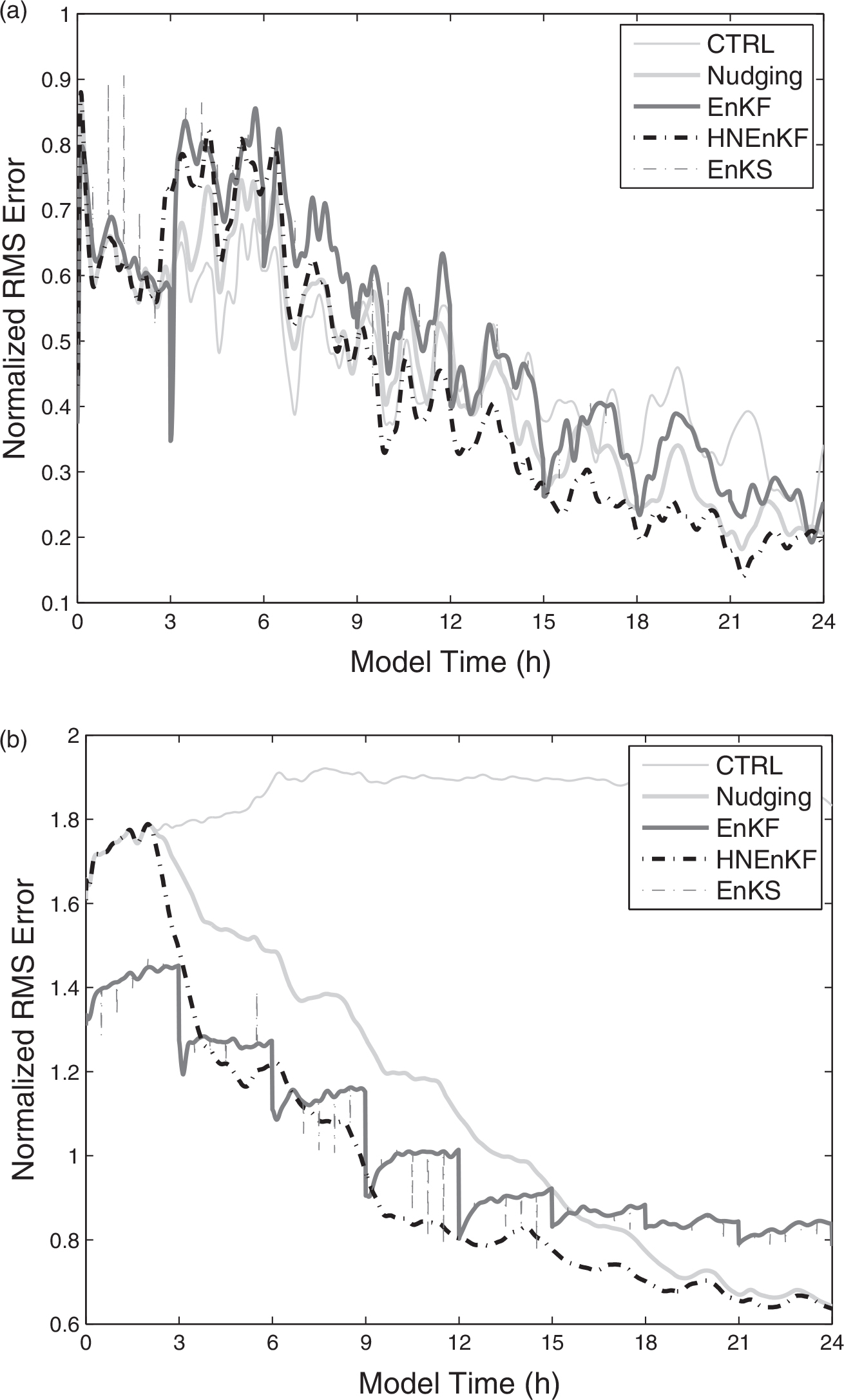
Fig. 4.
The sums of nudging tendency terms from eq. (5) at every grid point at the first observation time (3 h) of the baseline simulation. (a) Case I and (b) Case II. The left column shows the sums of the nudging terms for each equation u, v and h from Experiment Nudging, and the right column shows the sums of the three hybrid nudging terms for each equation u, v and h from Experiment HNEnKF.
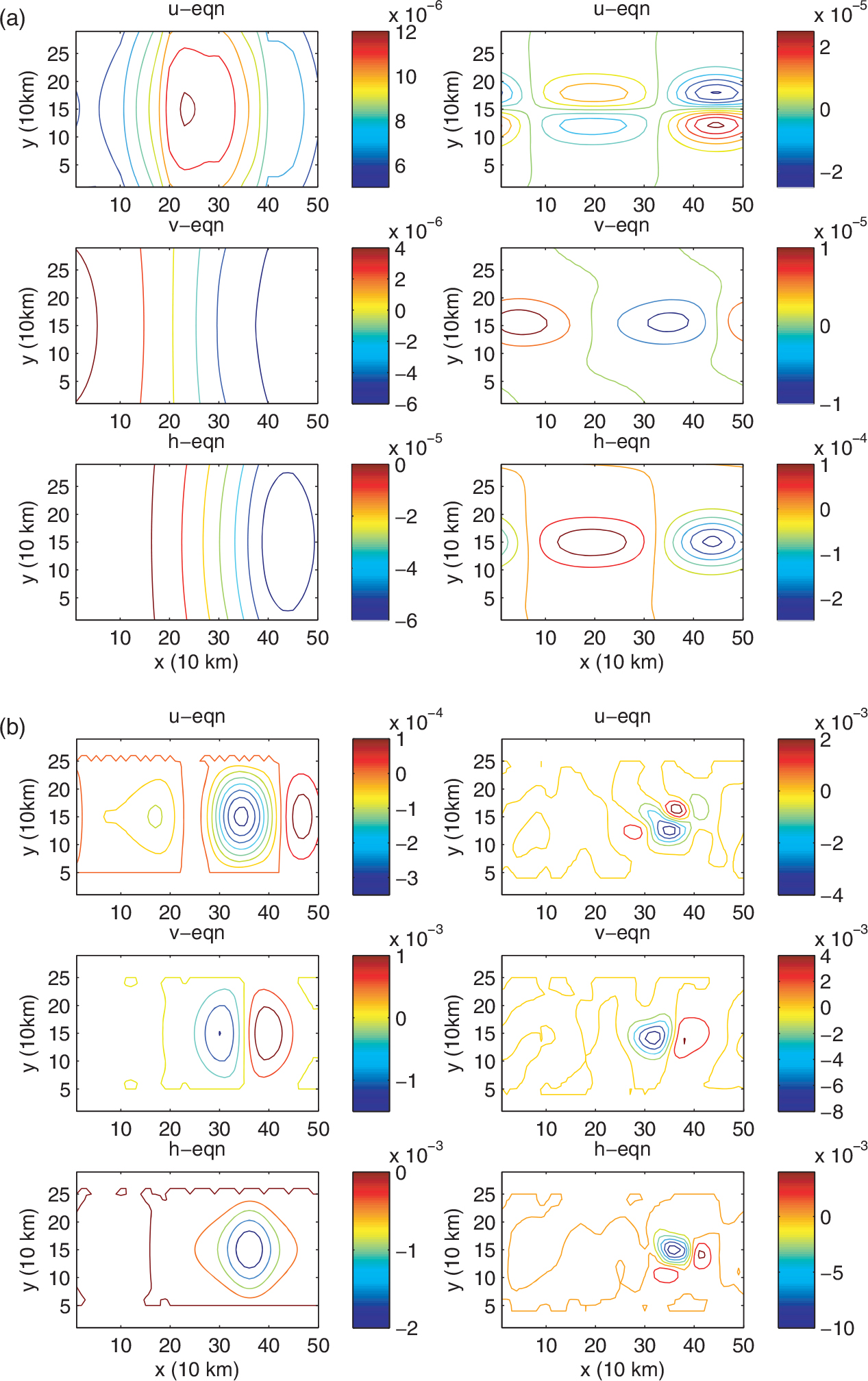
Fig. 5.
The height and wind fields of Case II at the end of the dynamic analysis using the baseline configuration. (a) Truth, (b) CTRL, (c) Nudging, (d) EnKF and (e) HNEnKF.
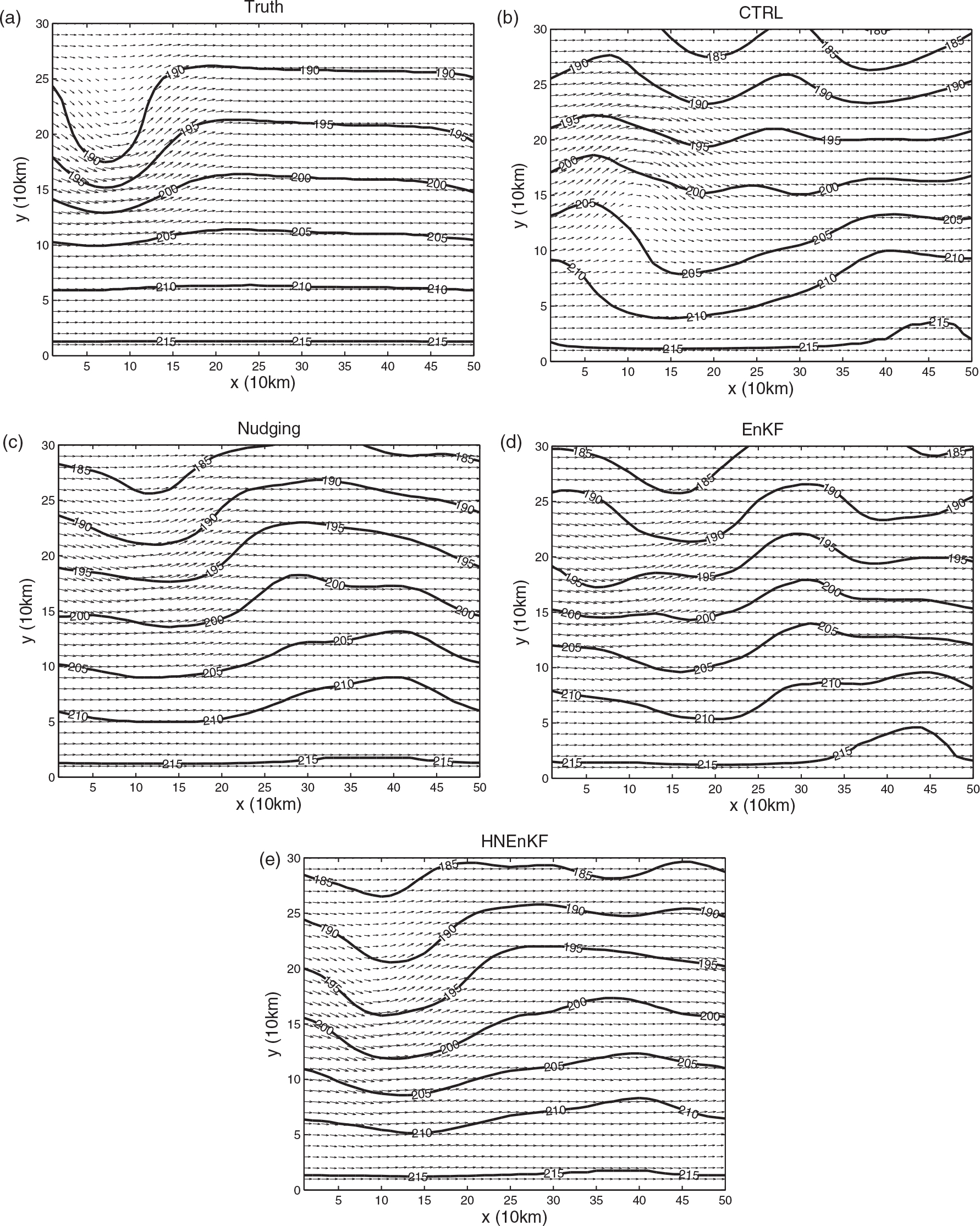
Fig. 6.
Height and wind RMS error and DP for Case I and Experiments Nudging, EnKF, HNEnKF and EnKS with different observation frequencies. (a) The average height RMS error, (b) the average height DP, (c) the average wind RMS error and (d) the average wind DP. Smaller values are better values for both average RMS error and DP.
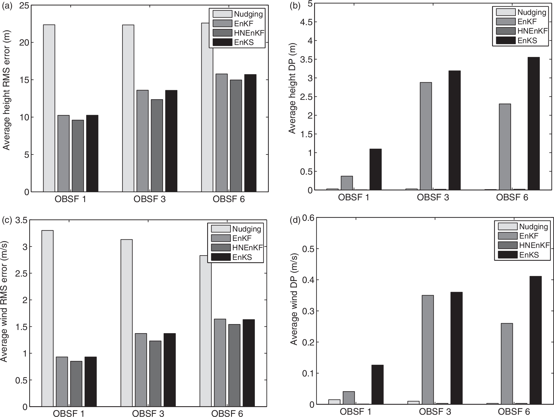
Fig. 7.
Same as Fig. 6, except for Case II.
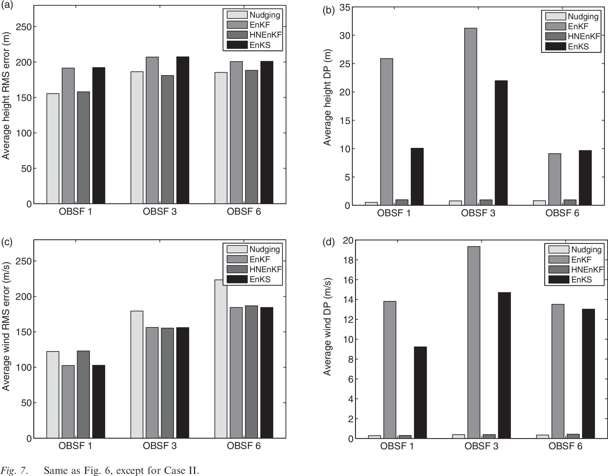
Fig. 8.
The height and wind fields of Case II at the end of the dynamic analysis for baseline configuration except using OBSF 1. (a) Nudging, (b) EnKF and (c) HNEnKF.
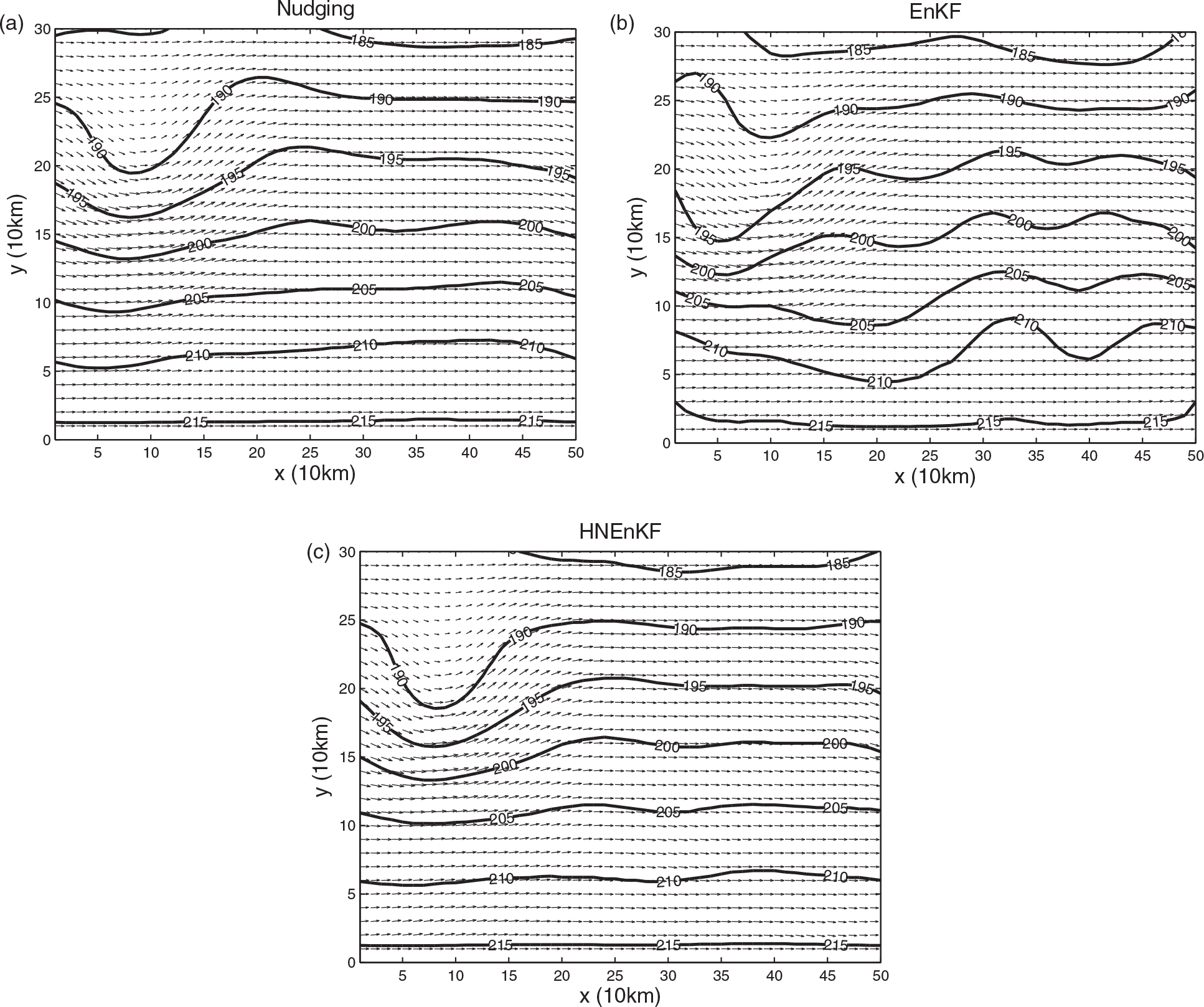
Fig. 9.
Height and wind RMS error and DP for Case I and Experiments Nudging, EnKF, HNEnKF and EnKS with different observation networks. (a) The average height RMS error, (b) the average height DP, (c) the average wind RMS error and (d) the average wind DP.
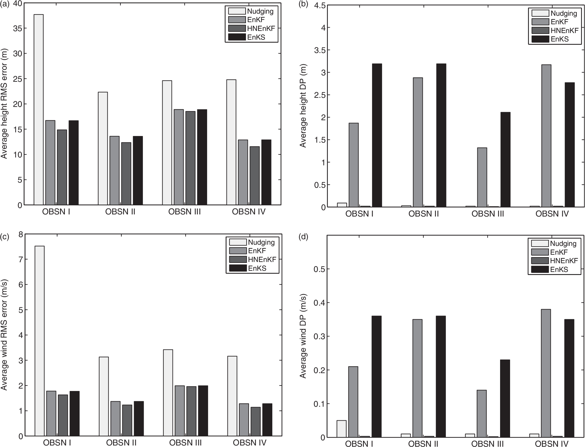
Fig. 10.
Same as Fig. 9, except for Case II.
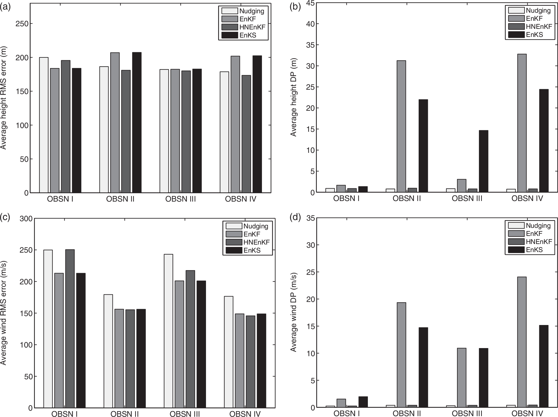
Fig. 11.
The height and wind fields of Case II at the end of the dynamic analysis for baseline configuration except using OBSN IV. (a) Nudging, (b) EnKF and (c) HNEnKF.
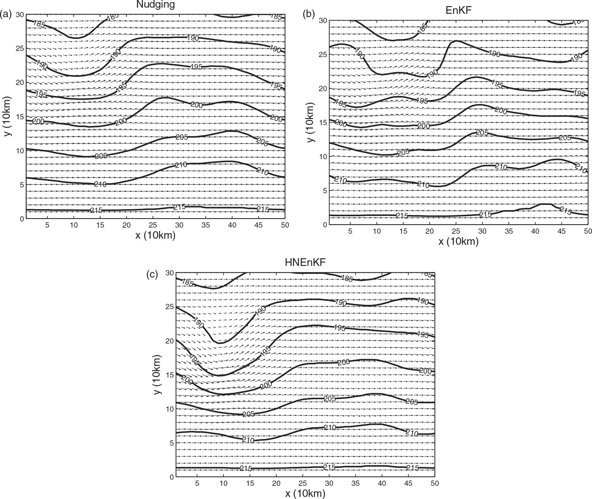
Fig. 12.
The range of ensemble spread and forecast error for the height and wind fields of the EnKF in Case I. (a) Height field with different observation frequencies, (b) wind field with different observation frequencies, (c) height field with different observation networks and (d) wind field with different observation networks.
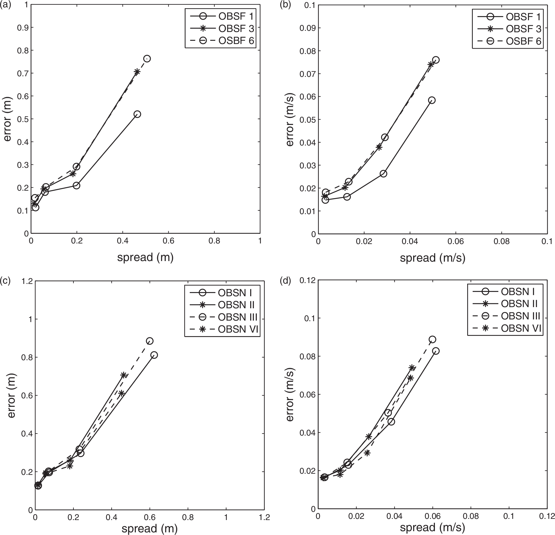
Fig. 13.
The same as Fig. 12, except for Case II.
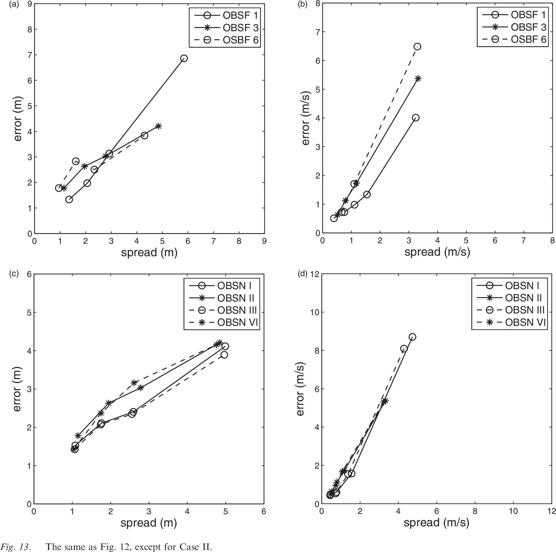
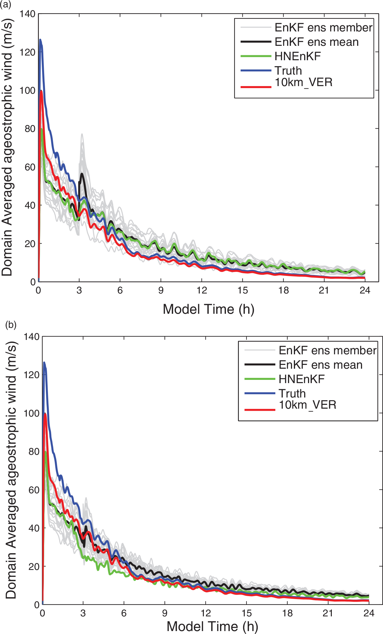
Fig. 14.
The domain-averaged ageostrophic wind computed for Case I for Experiments EnKF (each ensemble member in light grey, and the ensemble mean in black), HNEnKF (green), and the 1-km Truth (blue) and the 10-km_VER (red). (a) assimilating height observations only and (b) assimilating wind observations only.
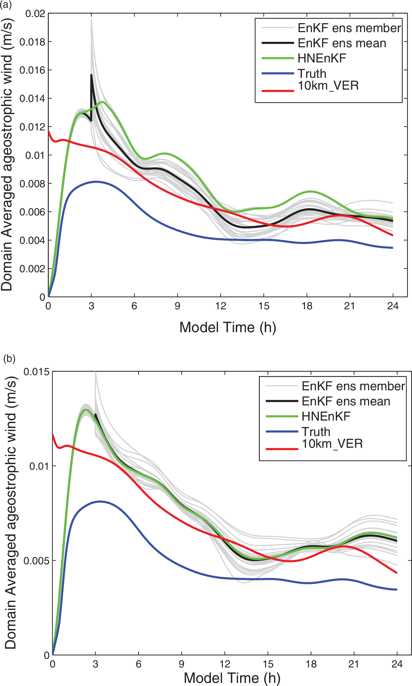
Fig. 15.
Same as Fig. 14, except for Case II.