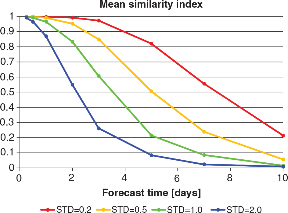
Fig. 1.
Schematic of the perceived forecast error verified against the analysis at the verification time t from two forecasts started from the analysis at t=0 h, and from the analysis at t=−6 h . Since the forecast started at t=−6 h serves as first guess for the analysis at t=0 h, the only difference between the two forecasts is the assimilation of the observations y 0 at t=0 h. Adapted from Langland and Baker (2004).
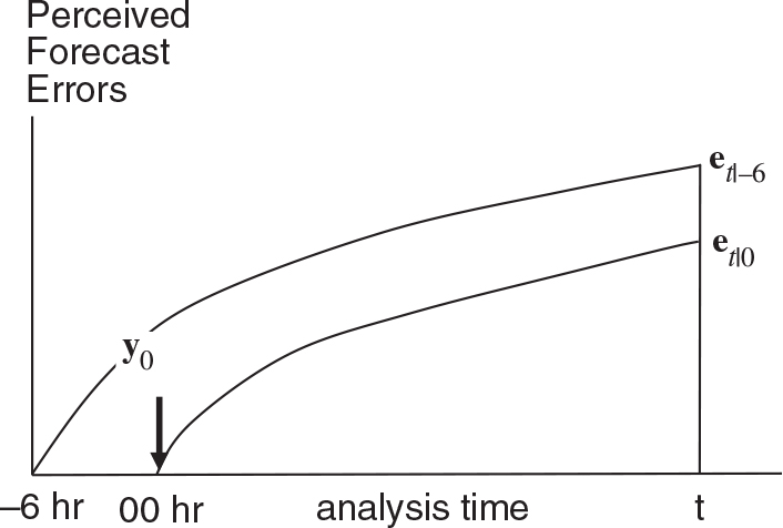
Table 1. Forecast error reduction of each formulation averaged over time and over 10 experiments. Truth and analysis show the average forecast error reduction verified against the truth, and against the analysis, respectively. Values in the parenthesis show the standard deviation of the 10 experiments. All values are multiplied by 100. No localization was used in the LETKF
Fig. 2.
Skill score of the estimation of the total forecast error reduction verified against the true forecast error reduction. Black, red and blue lines show the results of equations (4-ADJ), (5-OLD) and (6-NEW). The vertical error bars show the standard deviation of the 10 experiments. No localization was used in the LETKF.
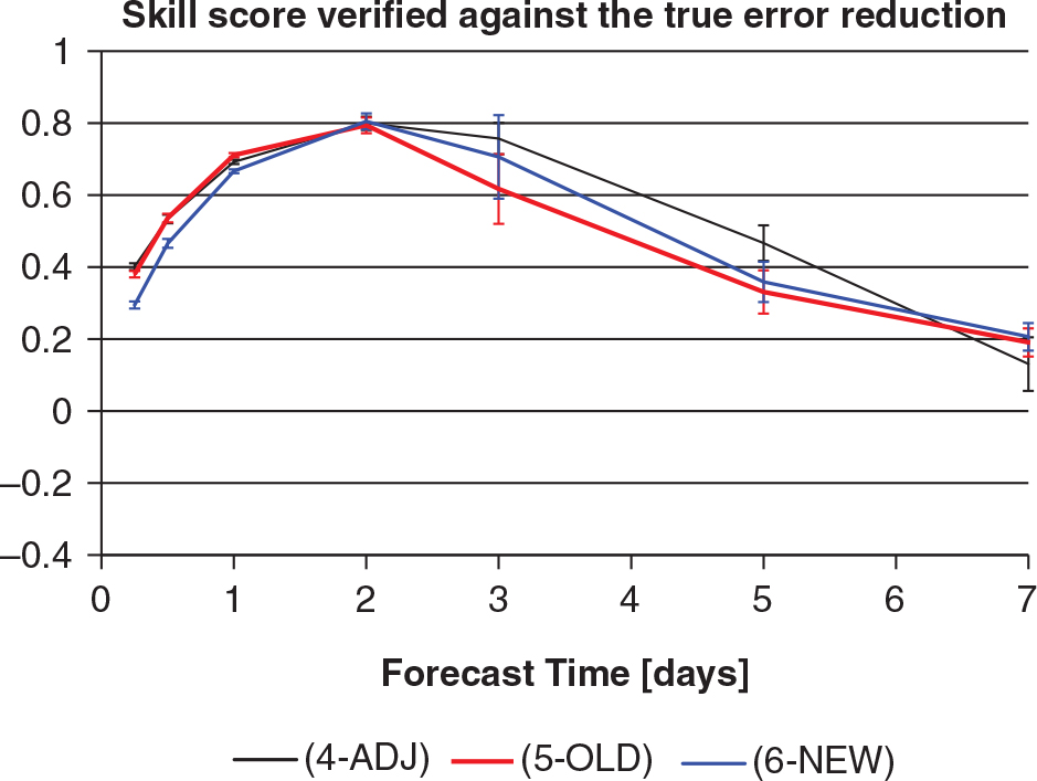
Fig. 3.
Same as Fig. 2 but with only 10 members and using localization in the analysis. No localization was applied for the ensemble-based observation impact computations.
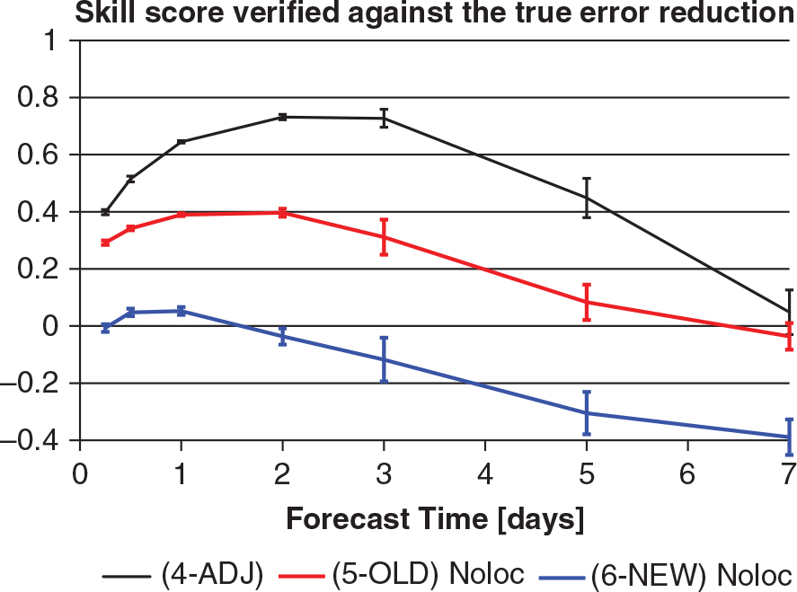
Fig. 4.
As per Fig. 3 but now with localization used in the observation impact computations. Red and blue lines show the results of equations (5-OLD) and (6-NEW) with a fixed localization (Fxloc) function as used in the LETKF analysis. Dotted green and light blue lines show the results of equation (6-NEW) with localization functions moving with non-linear evolution (NL-loc) and constant speed equal to the group velocity (CL-loc).
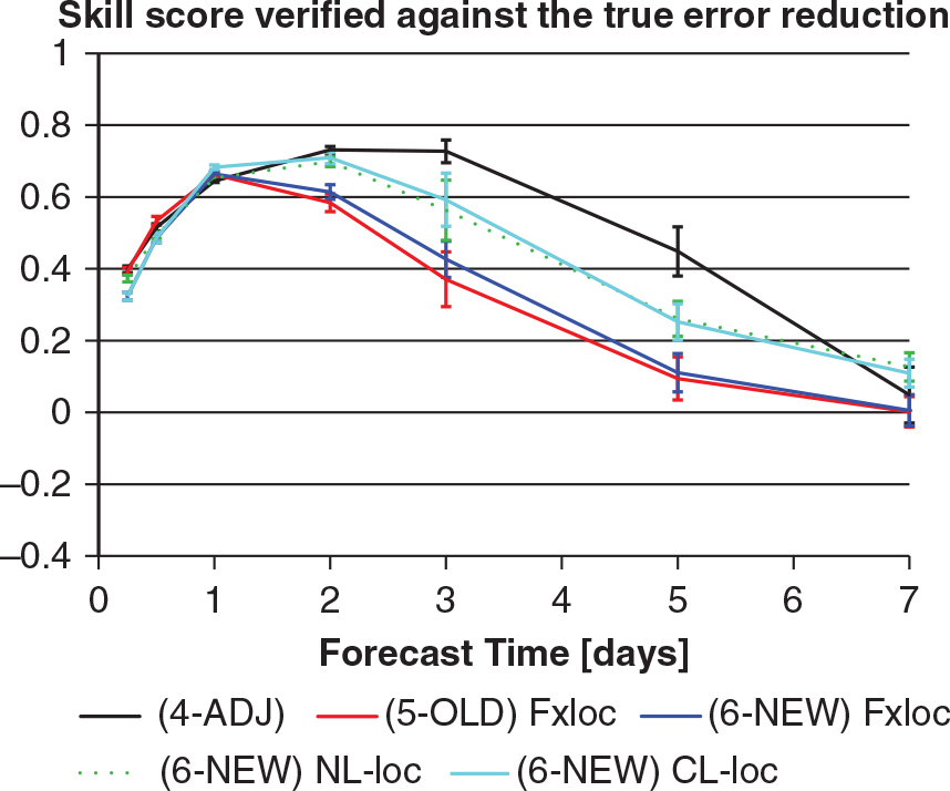
Table 2. Same as Table 1 but with 10 ensemble members and localization when indicated
Fig. 5.
Example of the evolution of the localization function with two methods. (a) Localization function with the non-linear incremental evolution (NL-loc); and (b) localization function moving with constant group velocity (CL-loc).
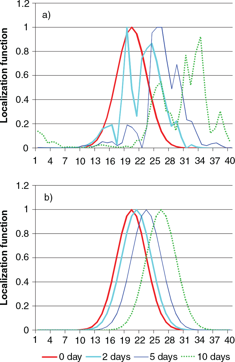
Fig. 6.
Time series of the total forecast error reduction at 5-d forecast from cycle 1000 to 1100. Pink lines show the true forecast error reduction, the black line is the adjoint estimation, the blue line is the ensemble estimation with fixed localization and the dotted green line is the ensemble estimation with non-linear evolution of the localization. A total of 40 observations are assimilated on each analysis time.
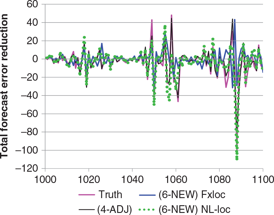
Fig. 7.
Fraction of the observations that are estimated to decrease the forecast error in each method. Purple solid line shows the result of data denial experiments, denoted as an Observing System Experiment (OSE).
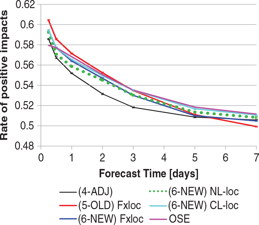
Fig. 8.
Time average of observation impact estimates at each point on 5-d forecast with (a) 1000 and (b) 100 samples, using the adjoint approach eq. (4), the LLK10 formulation eq. (5) and the new ensemble formulation eq. (6), both with fixed localization. The observation at grid point 11 has an error variance of 0.8 rather than the assumed value of 0.2.
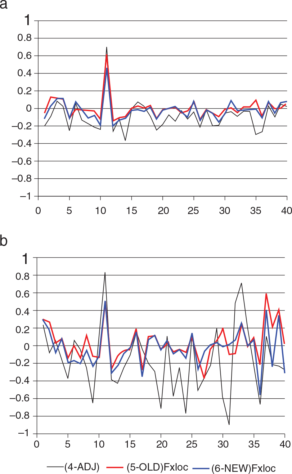
Fig. A1.
Similarity indices between the non-linear and tangent linear evolution of the perturbations. Standard deviation of the perturbations are 0.2 (red), 0.5 (yellow), 1.0 (green) and 2.0 (blue). Values are averaged over 1000 realizations.