Fig. 1.
Computational domain and the best track of Sinlaku.
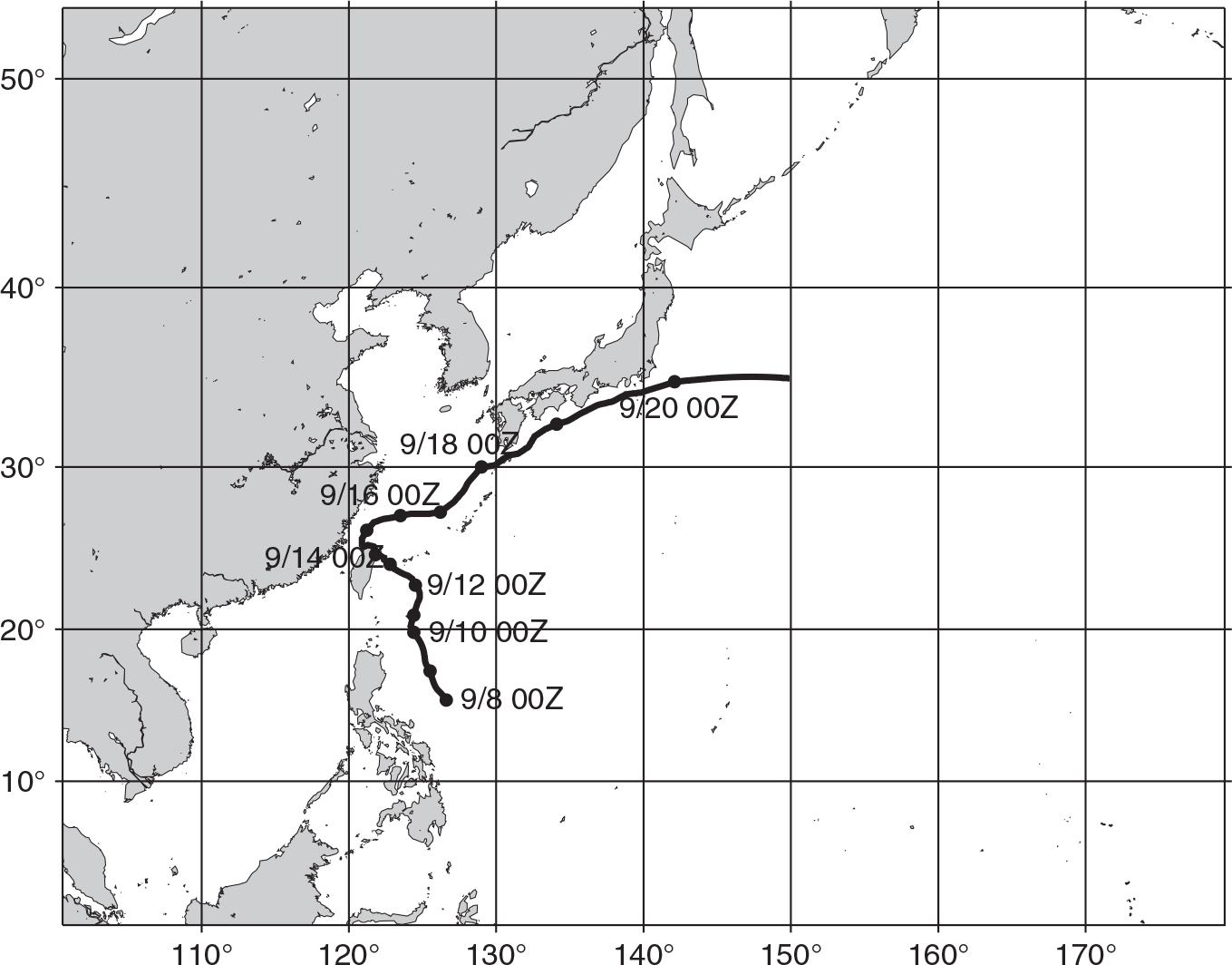
Fig. 2.
Adaptive inflation fields (contours enhanced by shading) and assimilated observations (marked as described in the legend) at the 15th model level (~500 hPa) at 0000 (top left), 0600 (top right), 1200 (bottom left), 1800 (bottom right) UTC on 12 September 2008. The legend shows the observing types with six-character codes as defined in PREPBUFR Table 1.a (Keyser, 2010), except for the closed circles showing AIRS data.
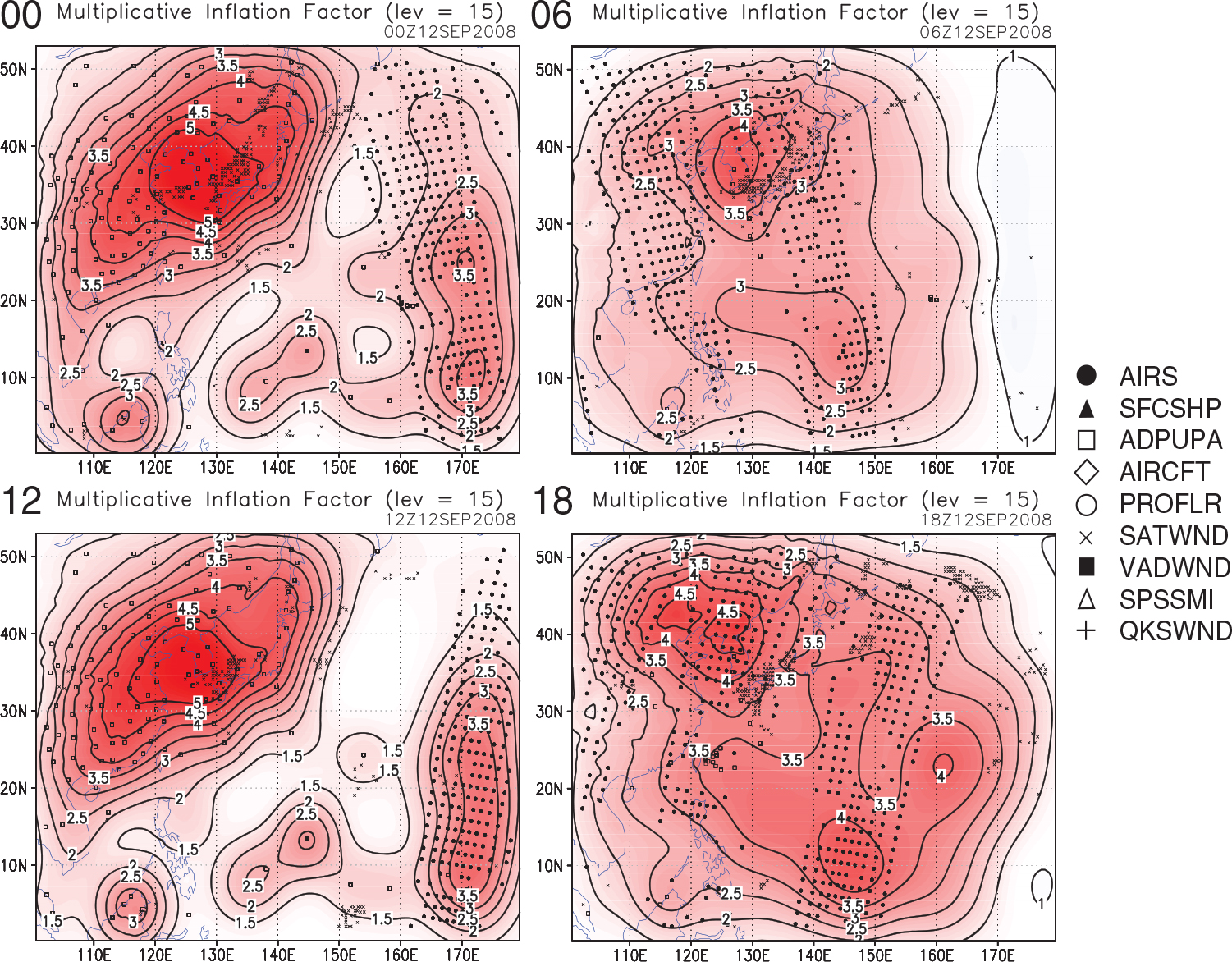
Fig. 3.
Mean differences (squares) and RMS differences (circles) of (a) temperature analyses (K) and (b) relative humidity analyses (%) for CTRL (dashed) and AIRS (solid) experiments relative to NCEP FNL, averaged over 27 days from 1 to 27 September 2008. Squares and circles indicate mean errors and RMSE, respectively.
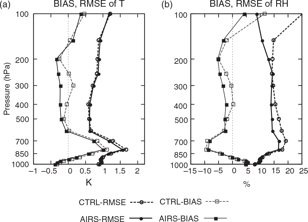
Fig. 4.
72 h forecast verifications relative to (a) radiosonde observations and (b) NCEP FNL for temperature (K) for CTRL (dashed) and AIRS (solid) experiments, averaged over 27 days from 1 to 27 September 2008. Squares and circles indicate mean errors and RMSE, respectively.
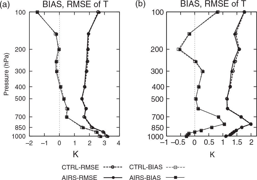
Fig. 5.
Relative improvement (%) of RMSE due to AIRS data for (a) zonal wind, (b) meridional wind, (c) temperature, and (d) specific humidity. The RMSEs are relative to radiosonde observations. The positive values (red) correspond to improvement due to AIRS data. The green box corresponds to Fig. 4 (a). The number of observations used for the verifications at each level is about 600, except for temperature and humidity at 1000 hPa which have about 300 observations.
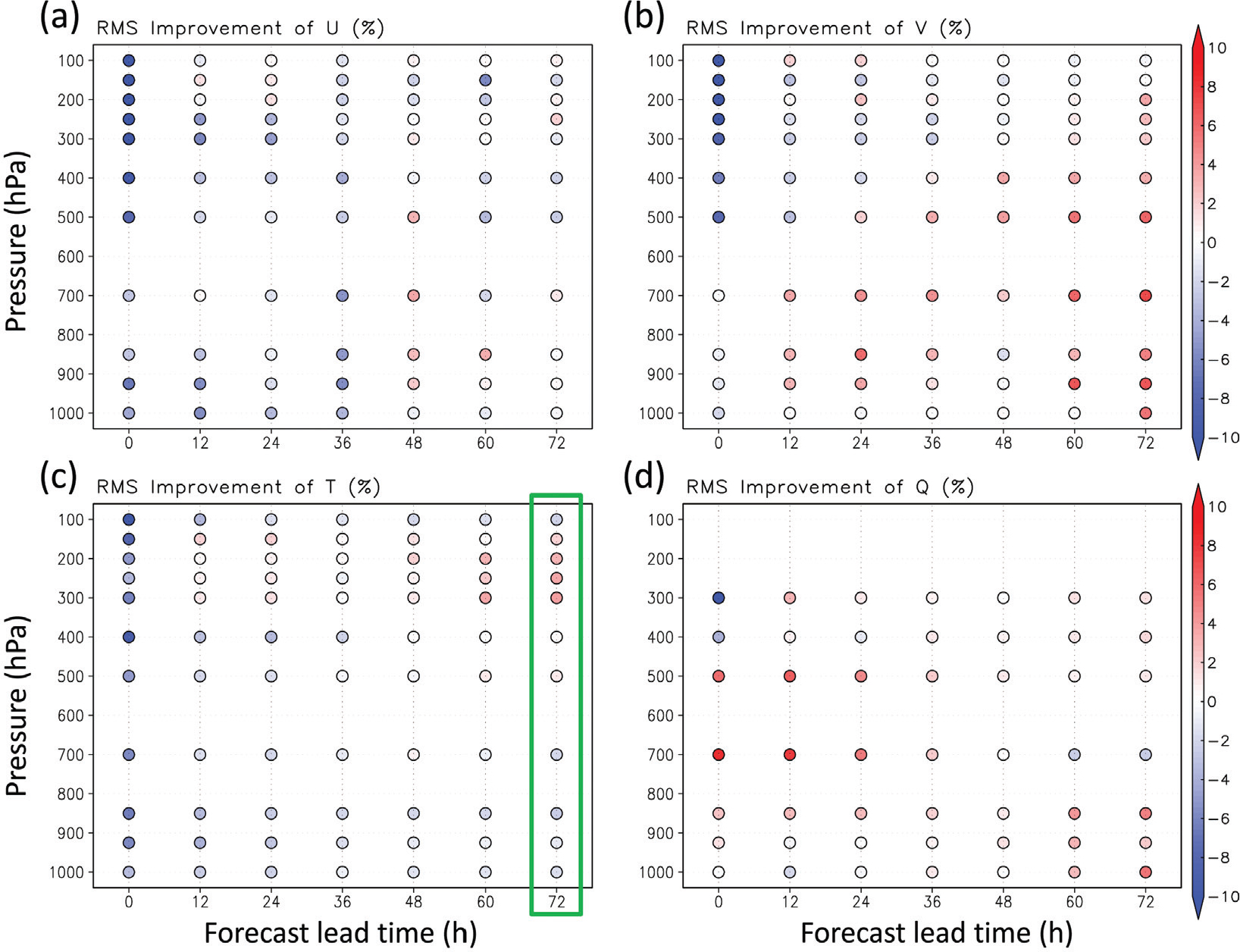
Fig. 6.
Similar to Fig. 5, but the RMSEs are relative to NCEP FNL, and (d) shows relative humidity instead of specific humidity. The green box corresponds to Fig. 4 (b).
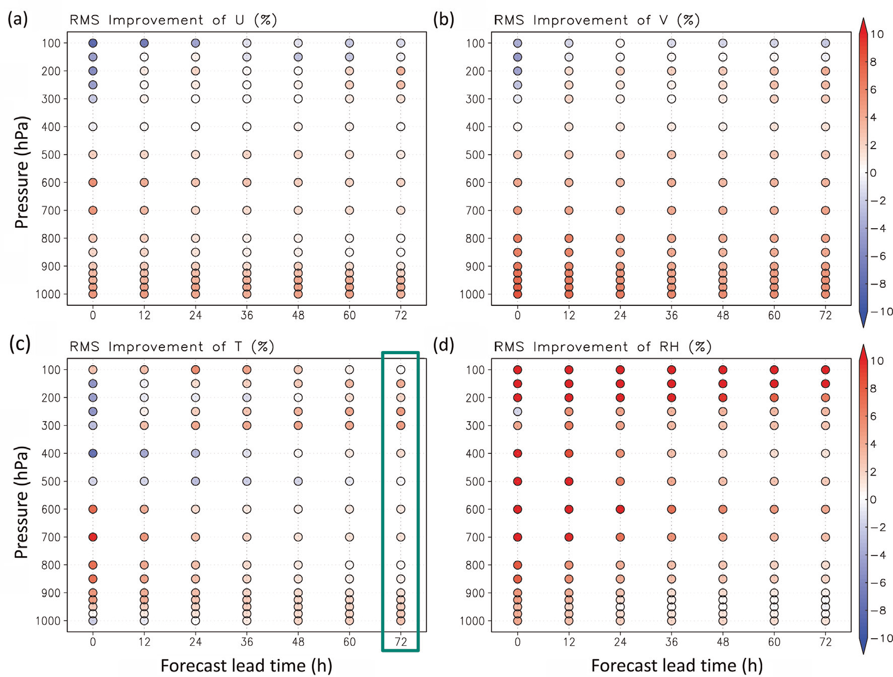
Fig. 7.
72 h forecast tracks of Sinlaku, initialised at 0600 UTC 12 September 2008 for the CTRL (blue) and AIRS (red) experiments. The black curve shows observed best track in the same period. Closed and open circles show the central position every 6 h.
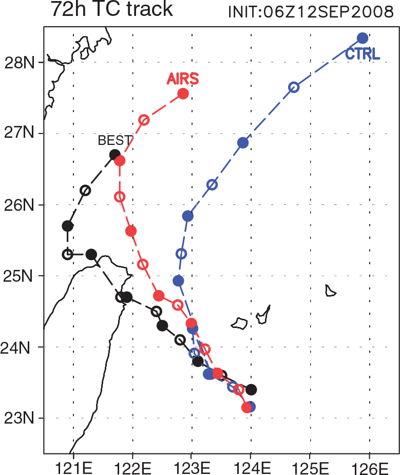
Fig. 8.
72 h forecast track errors (km) of Sinlaku of the CTRL (dashed) and AIRS (solid) experiments, averaged over 28 samples from 8 to 14 September 2008.
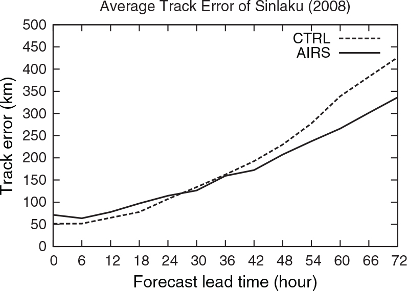
Fig. 9.
500 hPa geopotential height forecasts (m) at (a) 36 h and (b) 48 h forecast lead times initialised at 0600 UTC 12 September 2008 for the CTRL (blue) and AIRS (red) experiments.
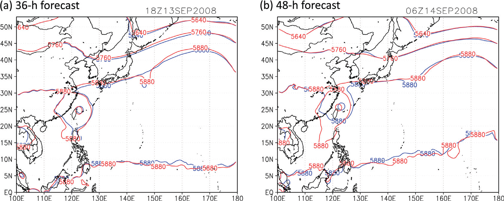
Fig. 10.
72 h minimum central pressure forecasts of Sinlaku of the CTRL (blue) and AIRS (red) experiments, each line corresponding to different initial times (total 28 initial times from 8 to 14 September). The observed best track is shown by the black line.
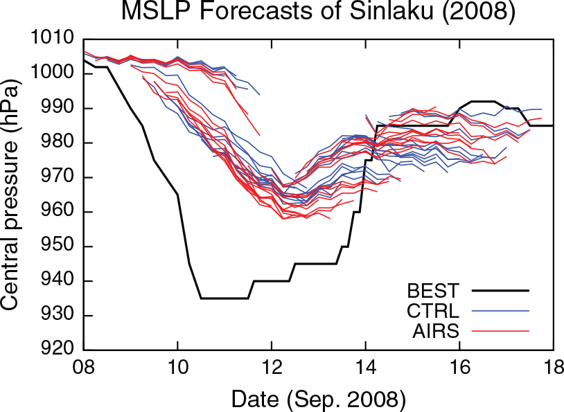
Fig. 11.
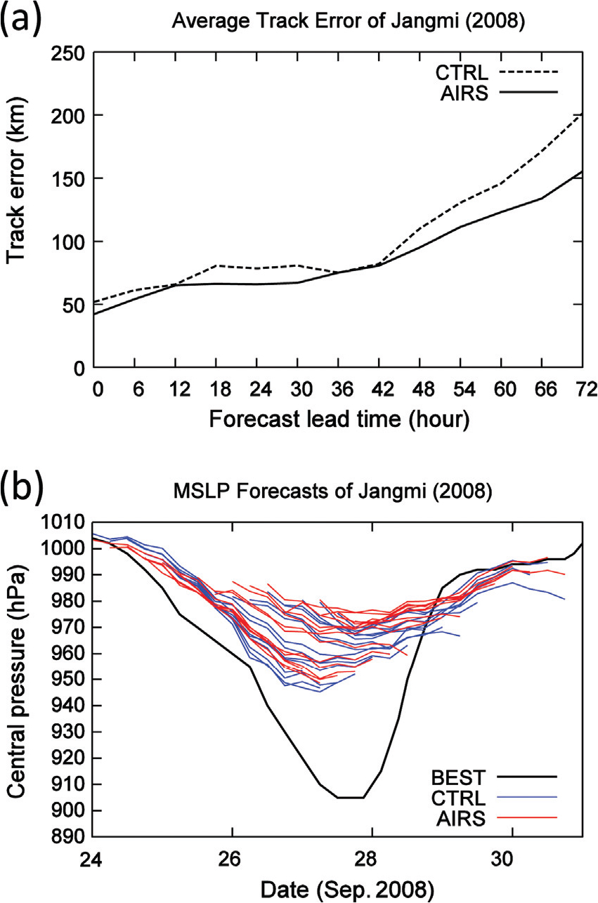
Similar to Figs. 8 and 10, but for Typhoon Jangmi (2008). (a) 72 h forecast track errors (km) averaged over 16 samples from 24 to 27 September, and (b) 72 h minimum central pressure forecasts, each line corresponding to different initial times (total 16 initial times from 24 to 27 September).