Fig. 4.
Rms analysis error versus κ. λ is fixed at 0.9. The blue, red and black curves show the global, regional and combined rms errors, respectively. The blue and red horizontal dashed lines show the global and the regional rms errors from the separate analysis method. The values were averaged over 40 000 analysis cycles discarding the first 1000 cycles.
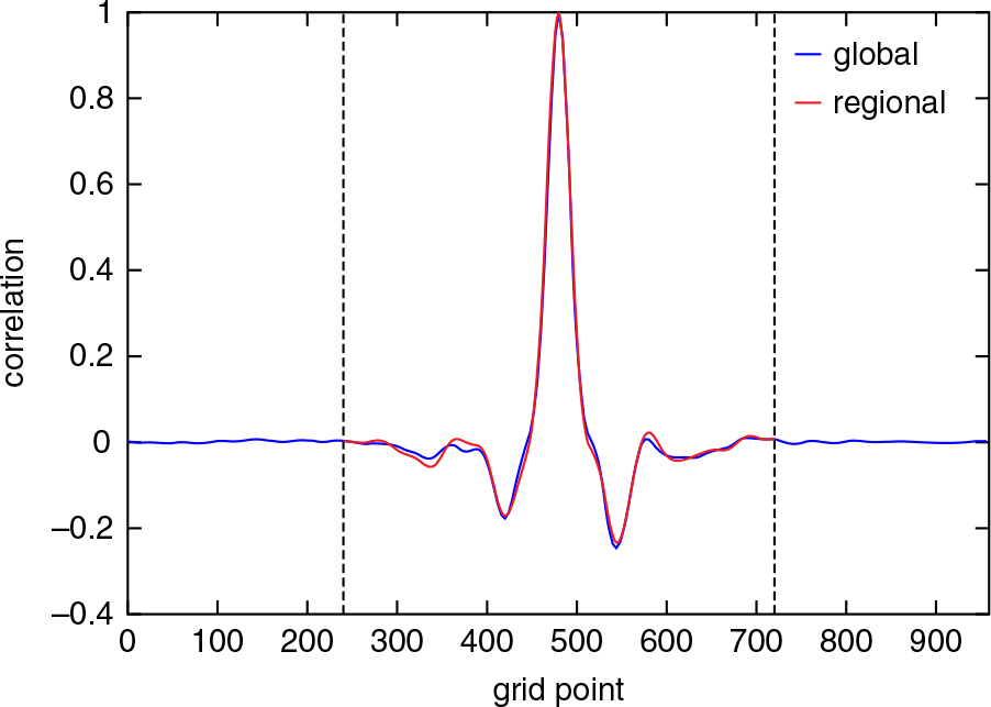
Fig. 7.
Rms analysis error versus κ with λ =0.7. A model error was introduced to the regional model by using F=14 in Lorenz model 3. The blue and red horizontal dashed lines show the global and the regional rms errors from the separate analysis method. The values were averaged over 80 000 analysis cycles discarding the first 1000 cycles.
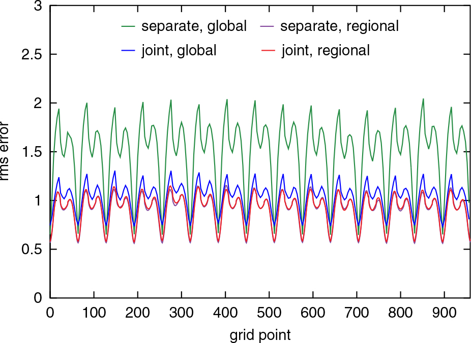
Fig. 1.
Correlations of the background ensemble of the joint-state method without localisation as a function of the grid point. Seven hundred and twenty ensemble members were used. The values were averaged over 20 000 analysis cycles.
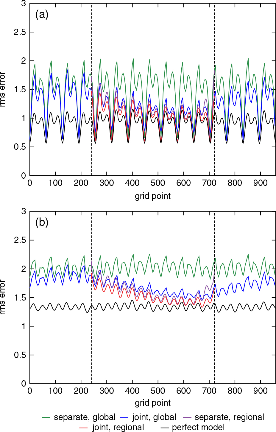
Fig. 2.
Rms analysis errors of the separate analysis and the joint-state analysis using the whole region for both the global and the regional models. In this and the subsequent figures, the rms error values were averaged over enough cycles to give stable values. In the case of present figure, the rms-error values were averaged over 100 000 analysis cycles, discarding the values of 1000 initial cycles. The green and the purple colours correspond to the global and the regional values obtained using the separate analysis method. The blue and the red colours correspond to the global and the regional values obtained using the joint-state method. The purple and the red lines are close to each other.
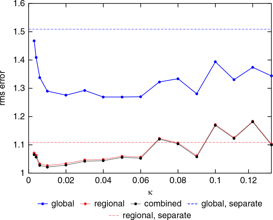
Fig. 3.
Rms errors of (a) the analysis (b) 1 d forecast of the separate analysis and the joint-state analysis. The colour scheme is the same as in Fig. 2. The additional black curves show the rms-error values when assimilations were done globally using the true model (Lorenz model 3). The two vertical dashed lines at grid points 240 and 720 indicate the boundaries of the subregion. The rms-error values were averaged over 100 000 analysis cycles.
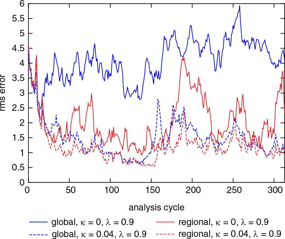
Fig. 5.
Rms analysis error versus analysis cycle. The solid blue and red correspond to the global and the regional rms errors when κ=0, λ=0.9. The dashed blue and red correspond to the global and the regional rms errors when κ=0.04, λ=0.9.
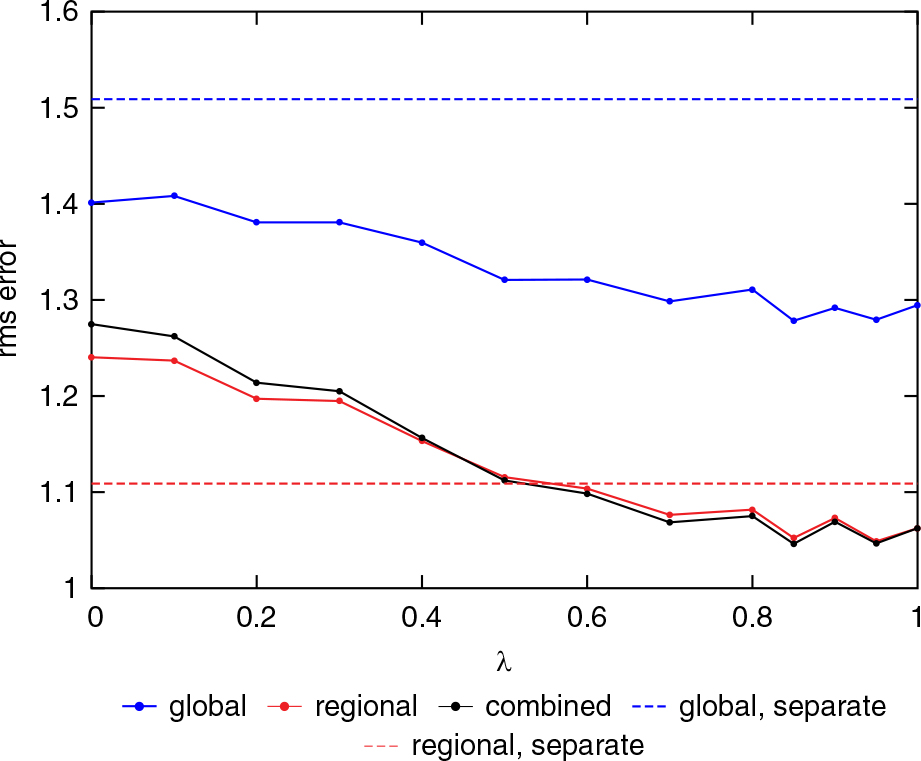
Fig. 6.
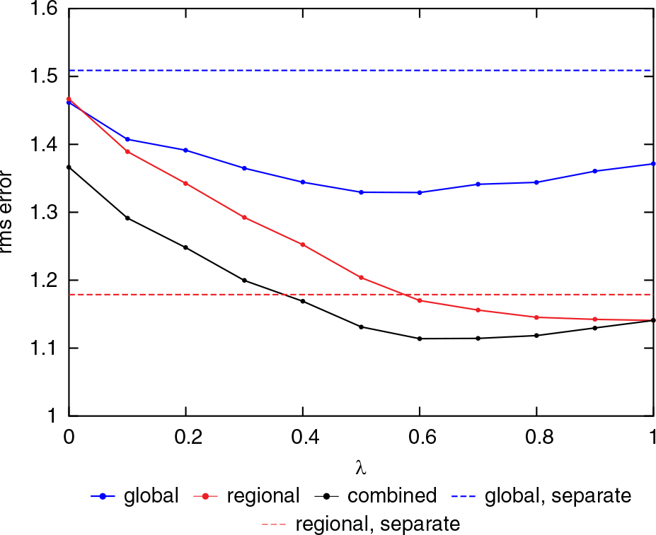
Rms analysis error versus λ. κ is fixed at 0.04. The blue, red and black curves show the global, regional and combined rms errors, respectively. The blue and red horizontal dashed lines show the global and the regional rms errors from the separate analysis method. The values were averaged over 200 000 analysis cycles discarding the first 1000 cycles.
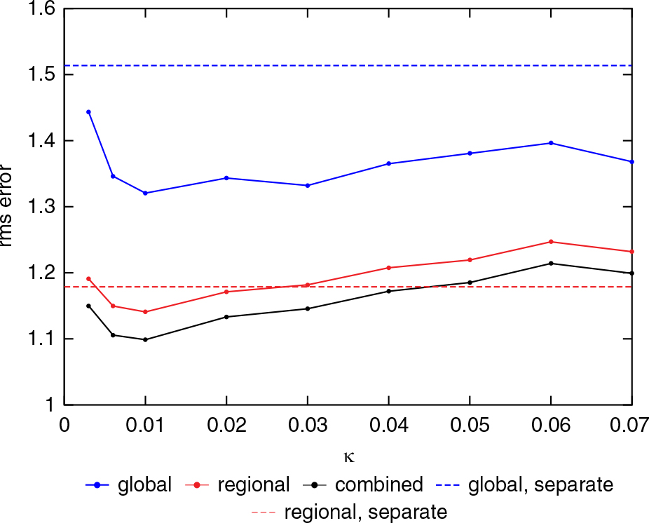
Fig. 8.
Rms analysis error versus λwith κ=0.01. A model error was introduced to the regional model by using F=14 in Lorenz model 3 for the regional model. The blue and red horizontal dashed lines show the global and the regional rms errors from the separate analysis method. The values were averaged over 200 000 analysis cycles discarding the first 1000 cycles.