Table 1. Experimental set-up for no-wind cases
Fig. 1.
Energetics at Ra = 107 (top) and Ra = 1010 (bottom). Specifically, (a) evolution of the energy budget at Ra = 107 with linear equation of state. At the later stages of the integration, the kinetic energy dissipation, ɛ, is equal to the conversion of potential energy to kinetic energy (C) which in turn is equal to the generation of potential energy by the thermodynamic forcing, P. (b) ɛ versus time for experiments with different equations of state at Ra = 107, and the upper bounds established by Paparella and Young (2002) and Nycander (2010). (c) Same as (a) but at Ra = 1010. (d) Same as (b) but only for linear equation of state. In all panels, the time is scaled by the diffusion time, H 2/κ where H is the total depth of the domain and κ is the diffusivity used in the experiment.
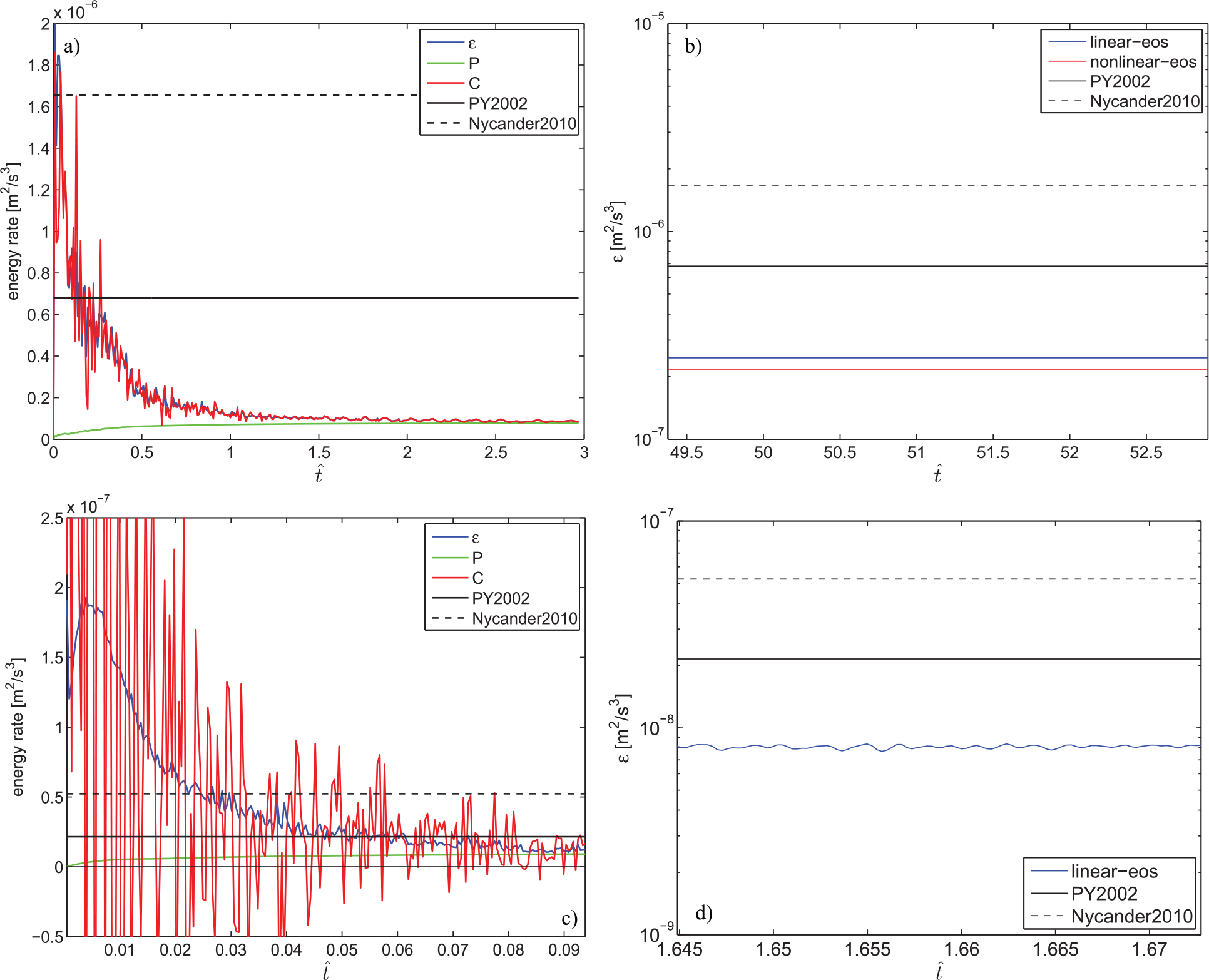
Fig. 2.
Time-averaged density field contours (left column) for and stream function (right column) for: (a) and (b) Ra = 106; (c) and (d) Ra = 107, (e) and (f) Ra = 108. At these Rayleigh numbers, the flow is almost steady, and snapshots are very similar.
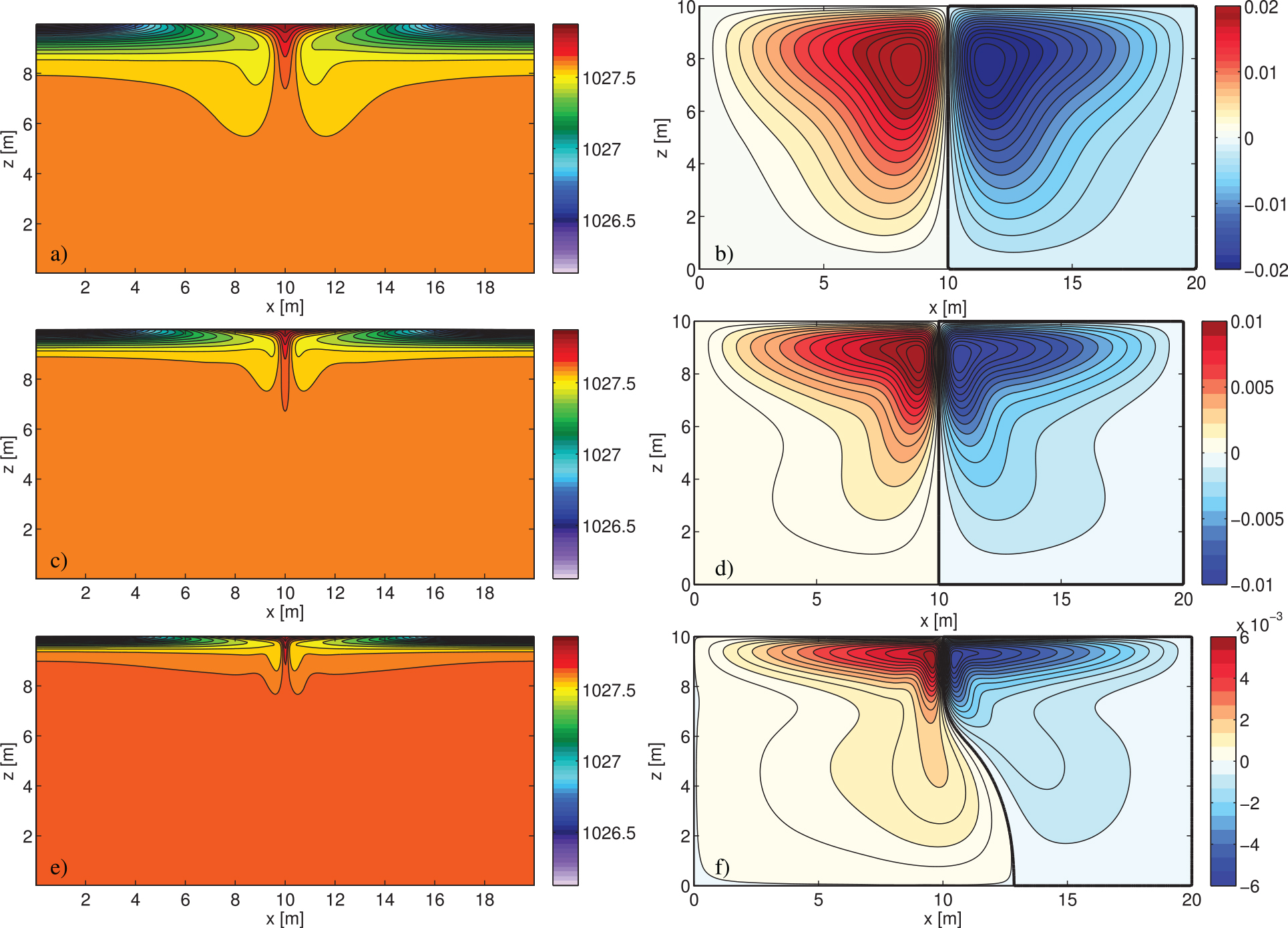
Fig. 3.
As for Fig. 2, but for Rayleigh numbers of, from the top: Ra = 109, Ra = 1010, and Ra = 1011. At Ra = 1010 and Ra = 1011, the flow is unsteady.
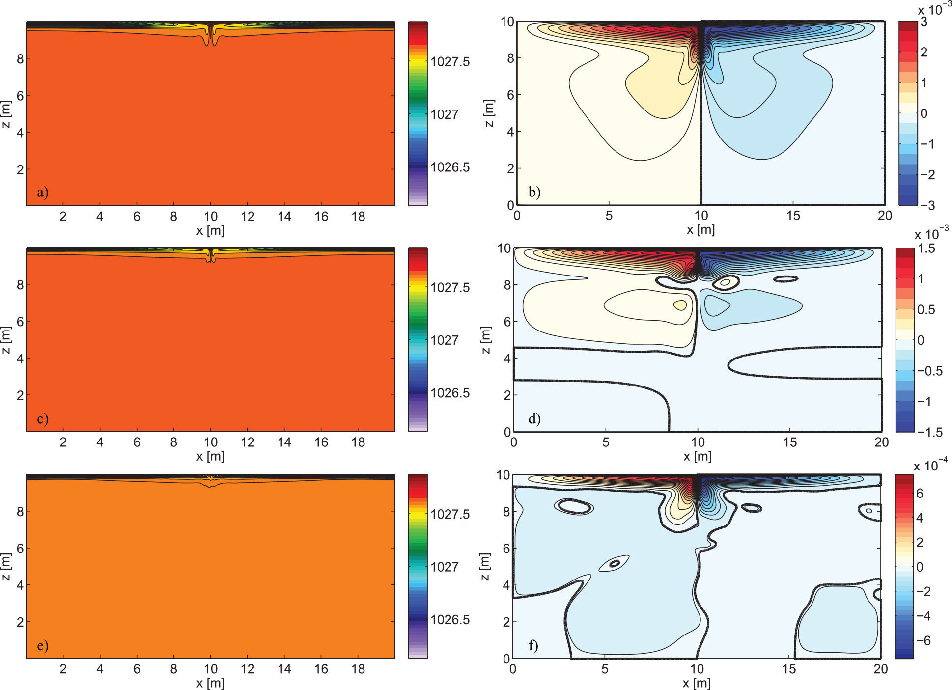
Fig. 4.
Snapshots of the density (left) and the stream function (right) fields of the Ra = 1010 experiment.
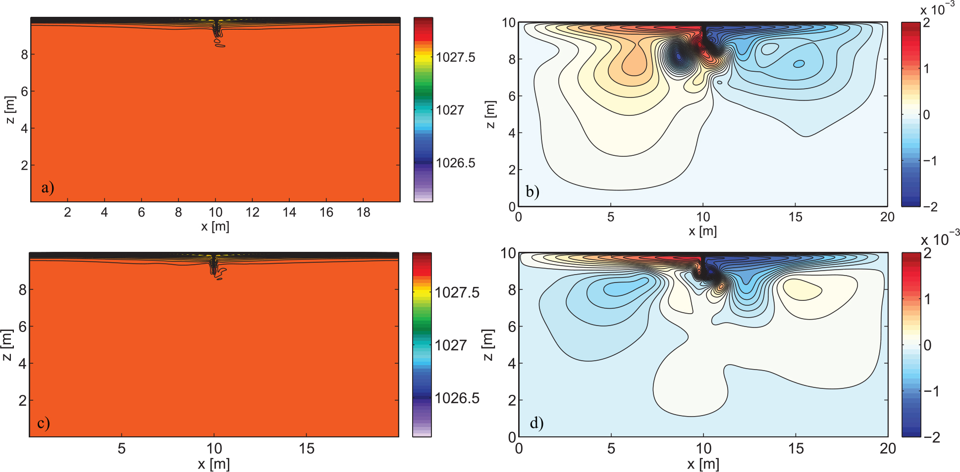
Fig. 5.
(a) Non-dimensional stream function () and dimensional stream function versus Rayleigh number, (b) Thermocline depth (h) versus Rayleigh number for no-wind experiments.
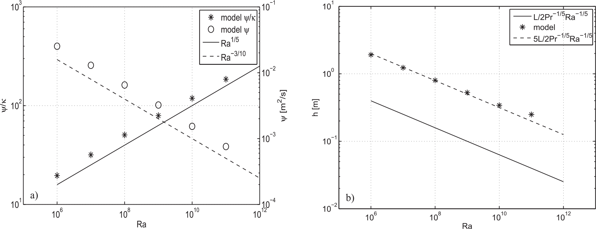
Fig. 6.
(a) The total kinetic energy of the flow for various values of the Rayleigh number is increased. Circles are the kinetic energy of the time-mean flow, and stars are the time-averaged kinetic energy of the total flow, including eddying terms. (b) Reynolds number, , as a function of Rayleigh number. (c) Total kinetic energy as a function of time for the Ra = 109, 1010 and 1011 cases. Time is scaled by the diffusion time, H 2/κ with κ the diffusivity at Ra = 1010.
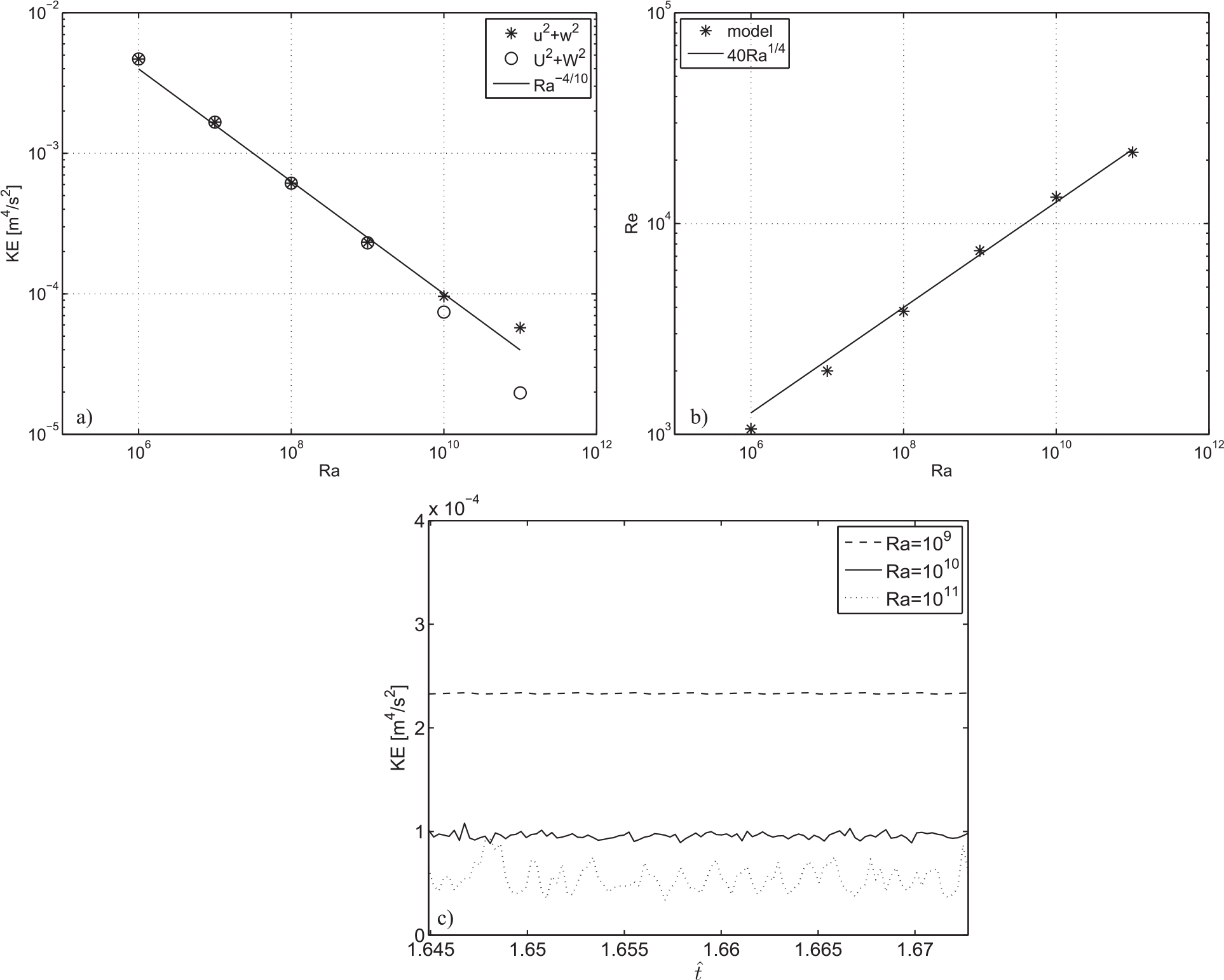
Fig. 7.
(a) Mean dissipation rate (ɛ) and non-dimensional dissipation rate () versus Rayleigh number. (b) Buoyancy variance dissipation rate (χ) as a function of diffusivity, κ.
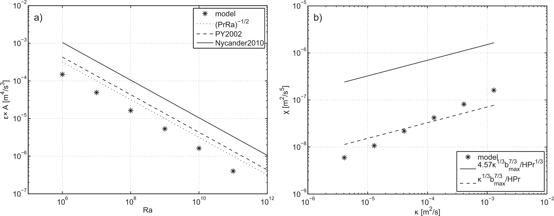
Fig. 8.
(a) Time-averaged density field contours (left column) for and stream function (right column) for: (a) and (b) at the top and at the bottom of the tank; (c) and (d) at the top and at the bottom of the tank.
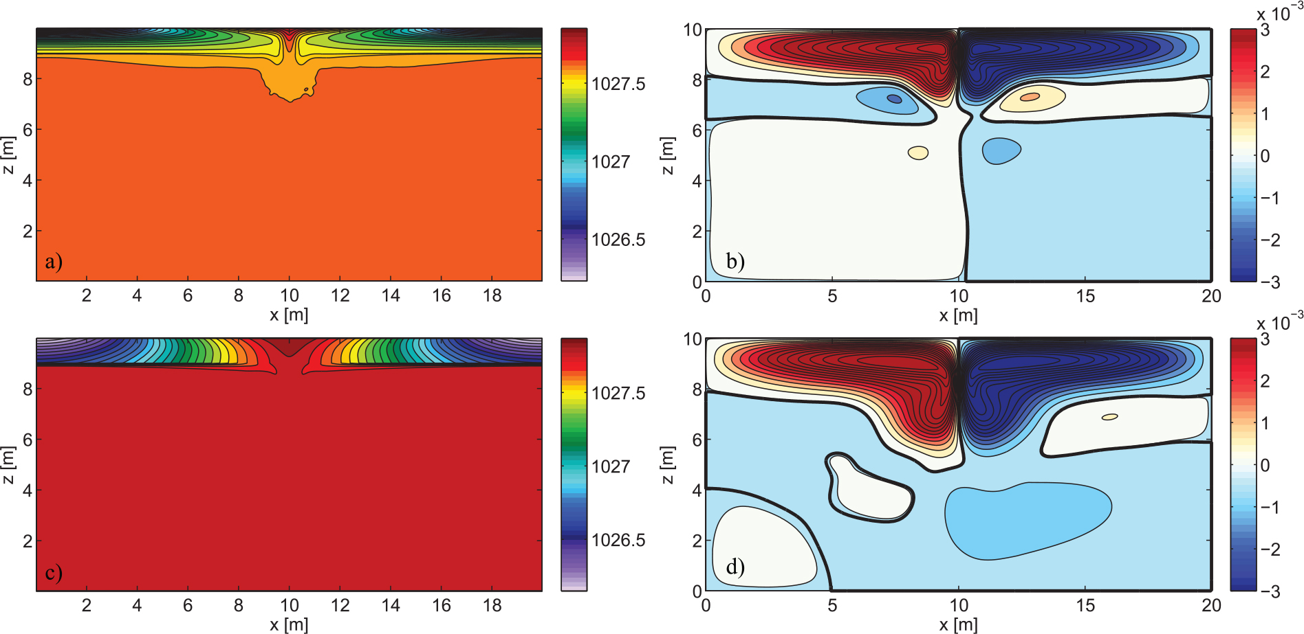
Fig. 9.
Time-averaged stream function fields at Ra = 107 for (a) linear equation of state, (c) nonlinear equation of state. Time-averaged density fields at Ra = 107 for (b) linear equation of state, (d) nonlinear equation of state.
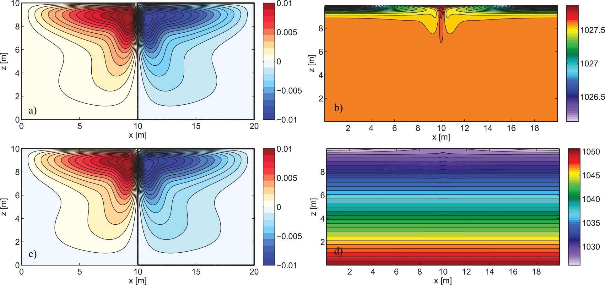
Table 2. Experimental set-up for wind cases
Fig. 10.
Time-averaged density field contours for (a) A 0=0.16, ω=0.008; (c) A 0=0.16, ω=0.04 and (e) A 0=0.16, ω=0.2. Time-averaged stream function contours for (b) A 0=0.16, ω=0.008; (d) A 0=0.16, ω=0.04 and (f) A 0=0.16, ω=0.2.
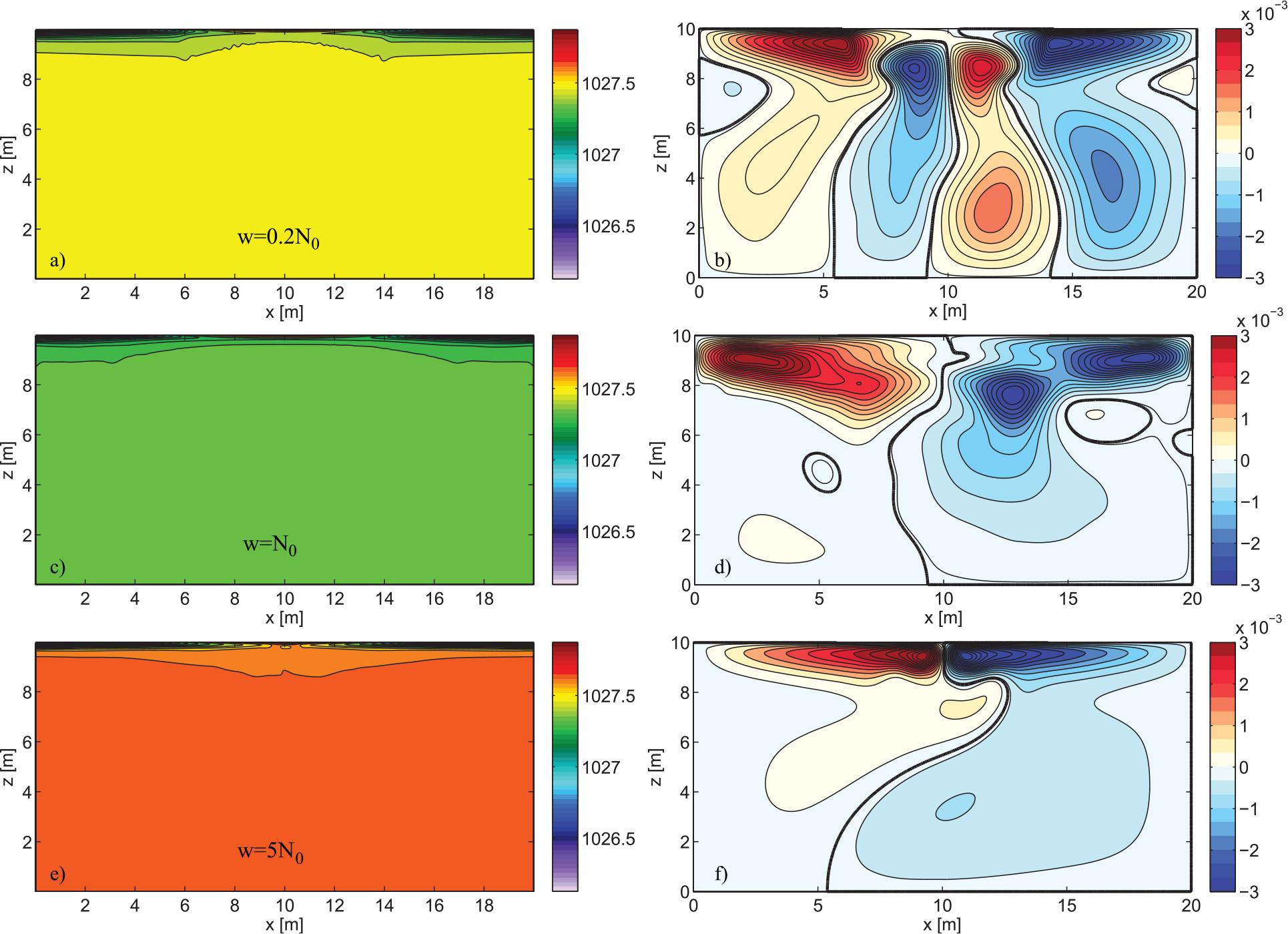
Fig. 11.
Time-averaged density field contours for (a) A 0=0.4213, ω=0.008; (c) A 0=0.4213, ω=0.04 and (e) A 0=0.4213, ω=0.2. Time-averaged stream function contours for (b) A 0=0.4213, ω=0.008; (d) A 0=0.4213, ω=0.04 and (f) A 0=0.4213, ω=0.2.
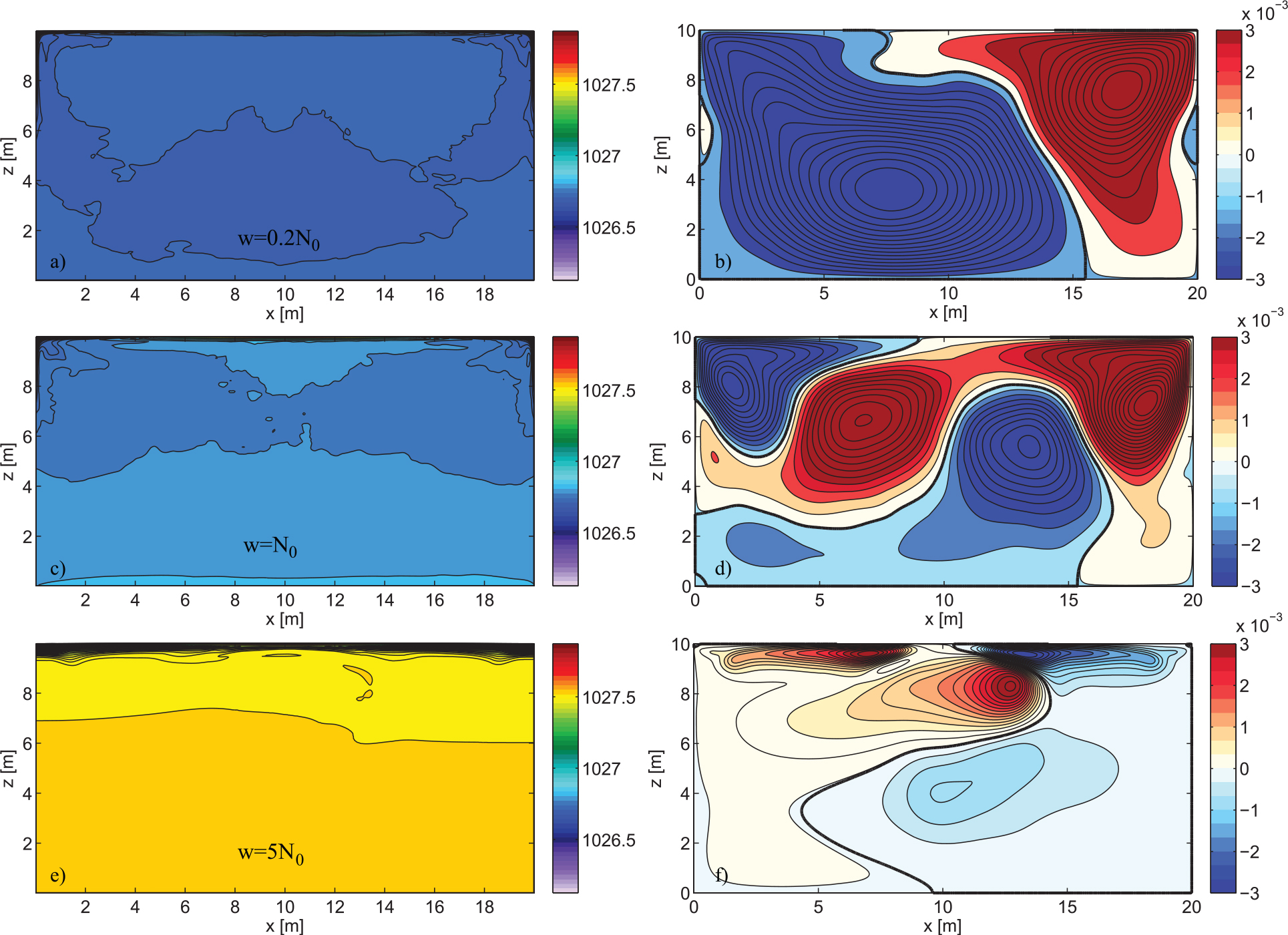
Fig. 12.
Spatial and time-averaged buoyancy profile for the no-wind case (solid line) and wind case (dashed line) with A 0=0.16 and ω=N 0, away from the sinking region. The straight vertical lines are the values at the bottom of the domain.
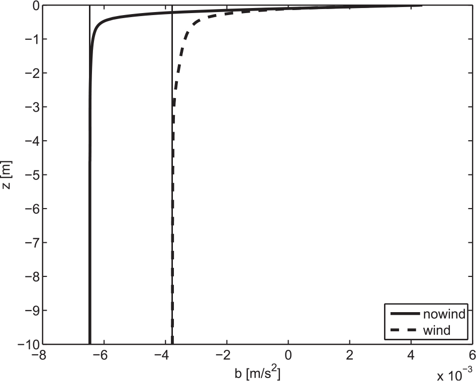
Fig. 13.
(a) Mean dissipation rate (ɛ) versus strength of the wind. (b) Buoyancy variance dissipation rate (χ) as a function of strength of the wind. (c) Maximum stream function versus strength of the wind.
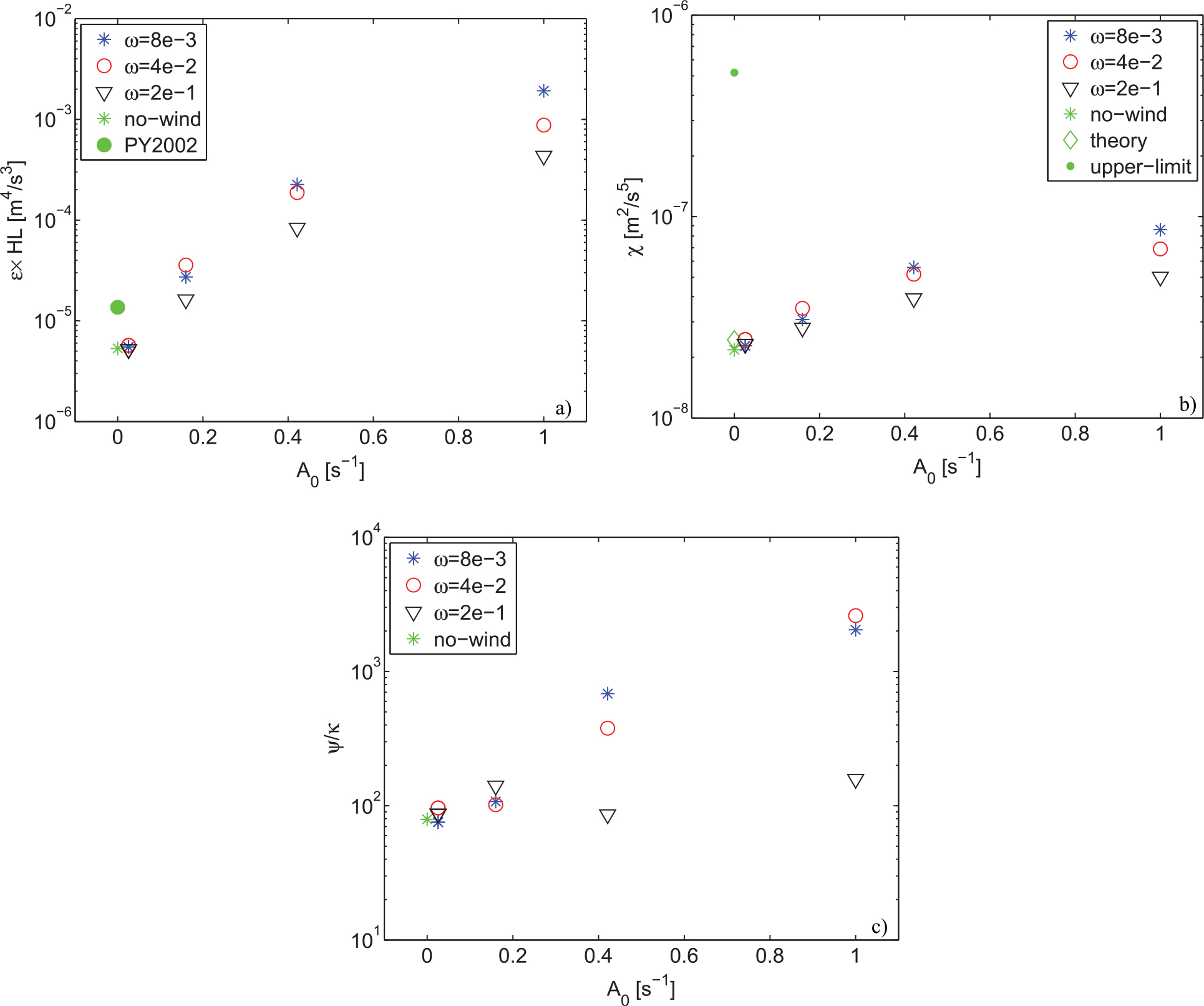
Fig. 14.
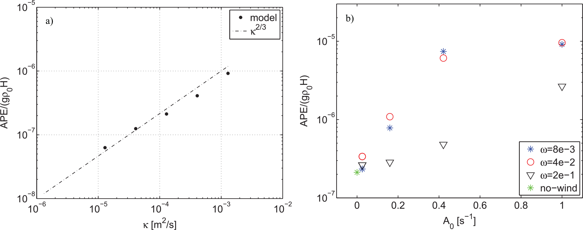
(a) Available potential energy as a function of diffusivity, κ. (b) Available potential energy versus strength of the wind.