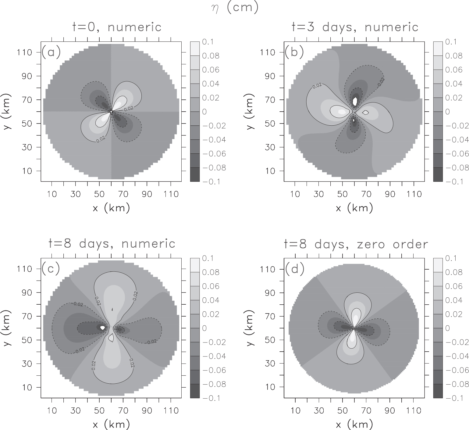
Fig. 1.
Linear (solid) and quadratic (dashed) topographies used for the simulation of topographic Rossby waves. Both profiles span the same height variation over the same latitudinal extent. Here, H 0=170 m.
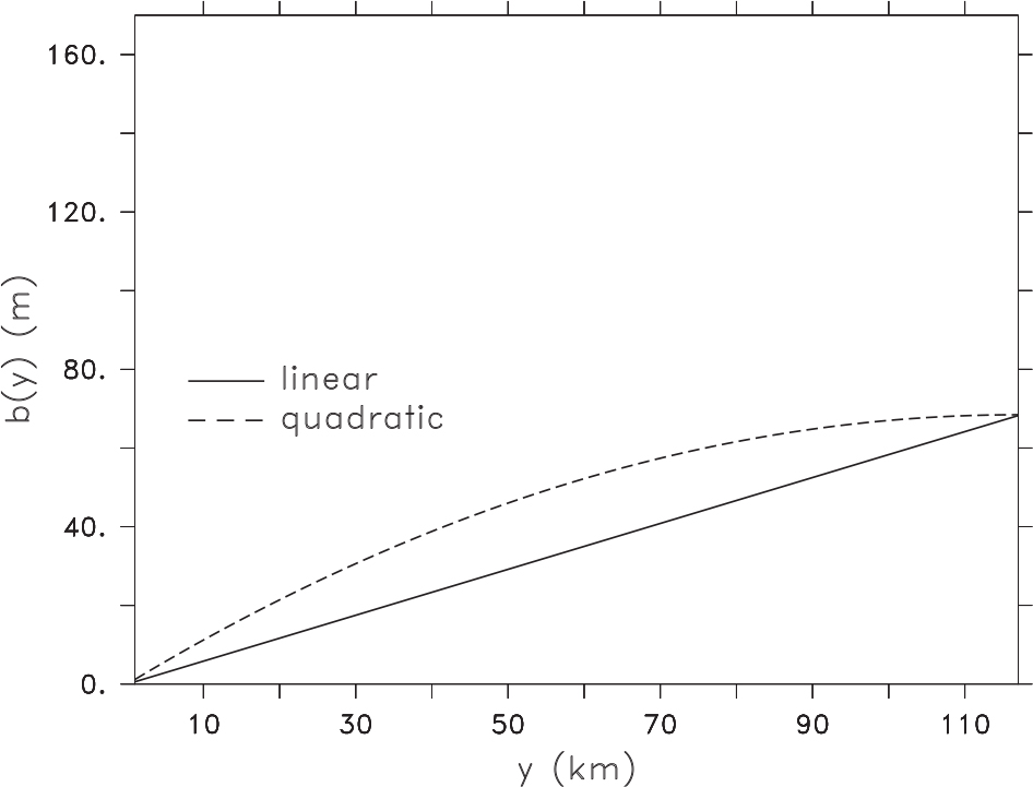
Fig. 2.
The initial (a) free surface η, (b) zonal velocity u and (c) meridional velocity v for the linear bottom topography case. The corresponding fields of the quadratic bottom topography are very similar to the linear topography ones. Note that the proportion of the figure does not reflect the same zonal and meridional extent. Also note that the meridional wavelength is four times larger than the zonal one.
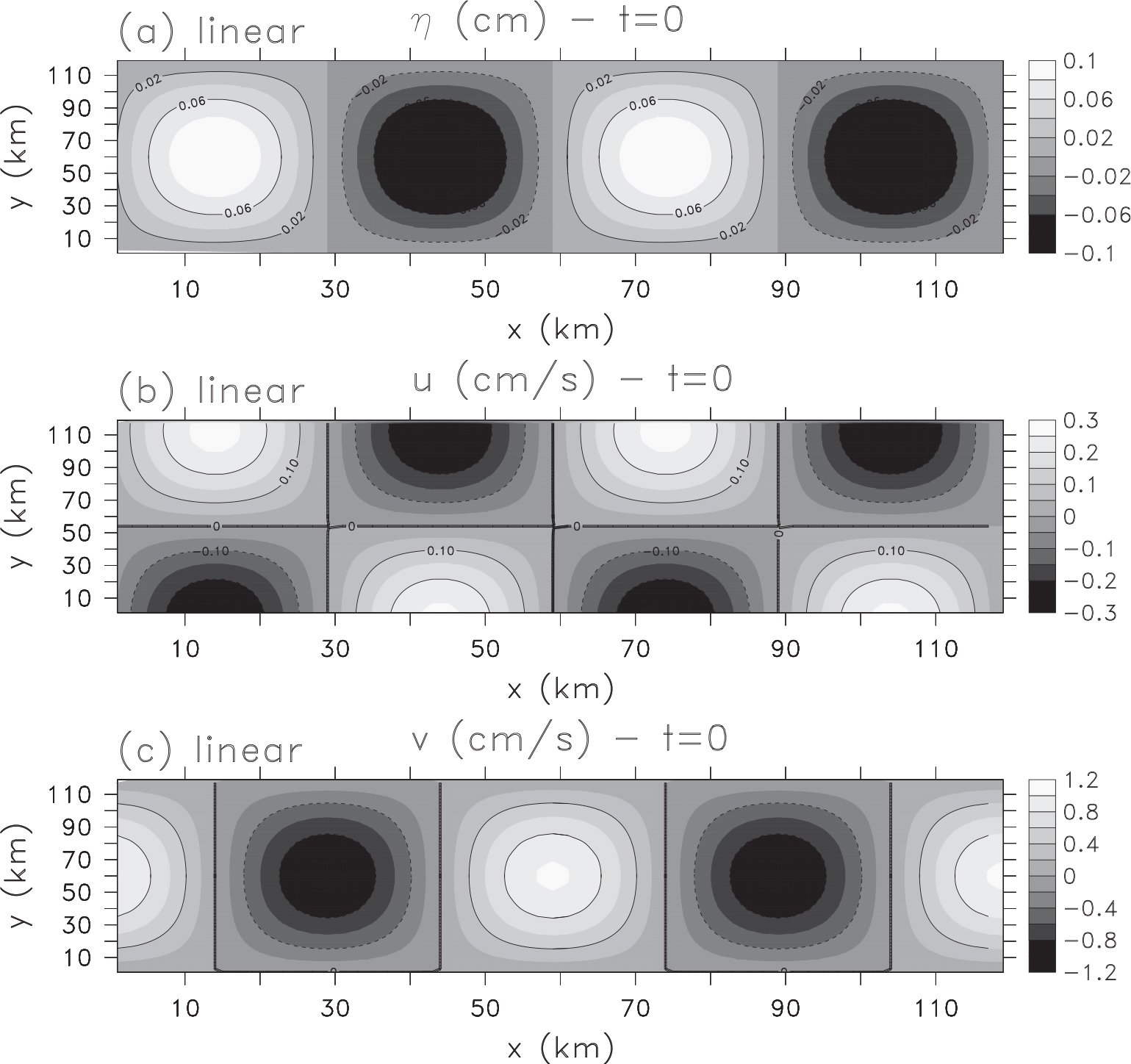
Fig. 3.
The numerical (upper panels), zeroth-order approximation (middle panels) and first-order approximation (lower panels) free surface η after 7 d of simulation, for the linear (left panels) and quadratic (right panels) bottom topographies. The agreement between the numerical and analytical results is good. In all cases, the wave propagates westward (such that the shallower depths are on the right), where for the linear bathymetry case, faster wave propagation is observed at higher latitudes.
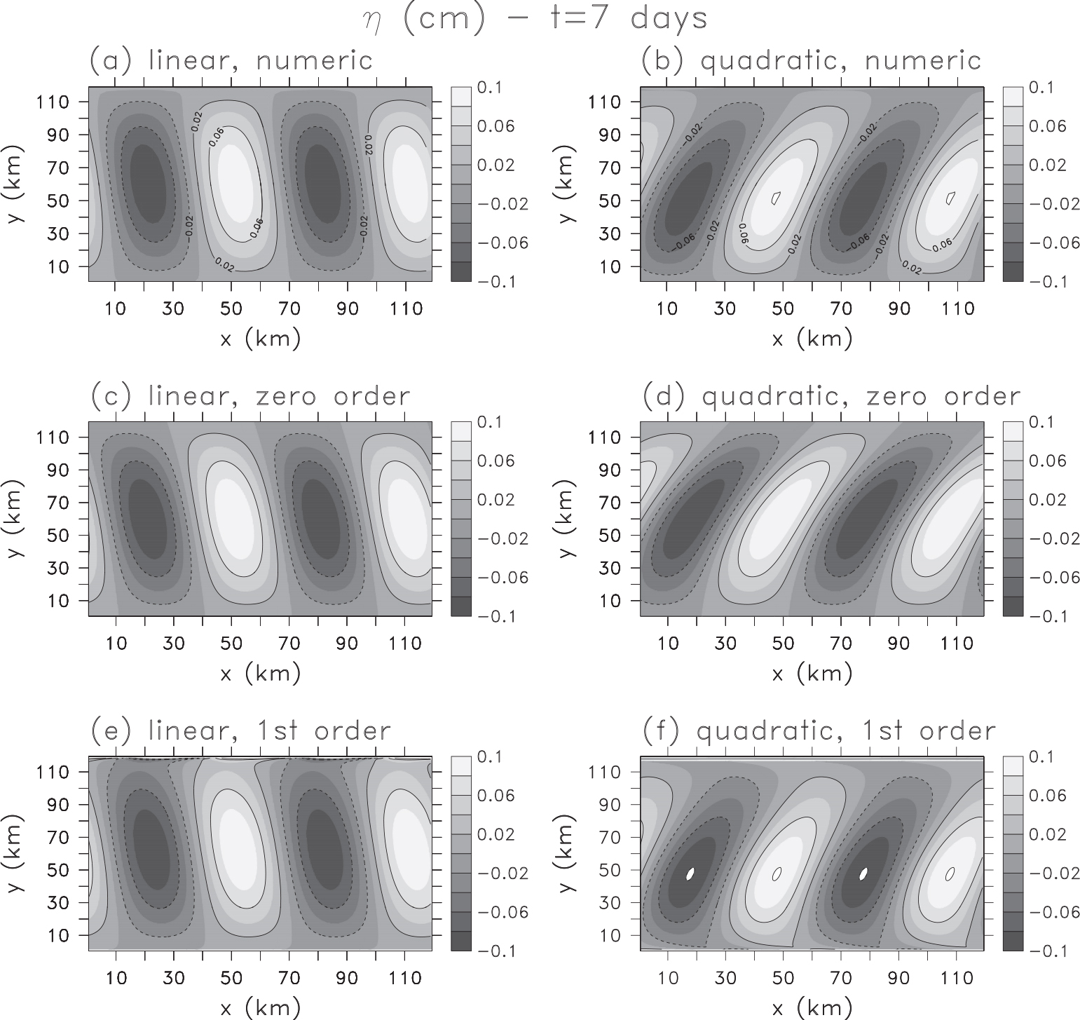
Fig. 4.
As Fig. 3 for the zonal velocity u. Note the large amplitude close to the boundary of the channel (small and large y). The first-order approximation (lower panels) is more similar to the numerical results (upper panels) compared to the zero-order approximation (middle panels).
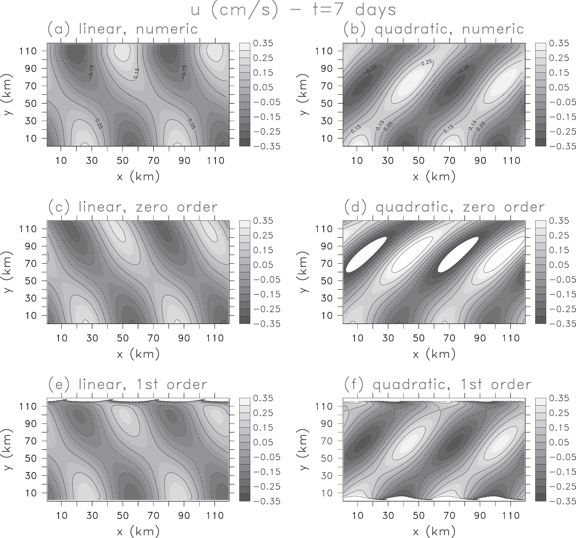
Fig. 5.
As Fig. 3 for the meridional velocity v.
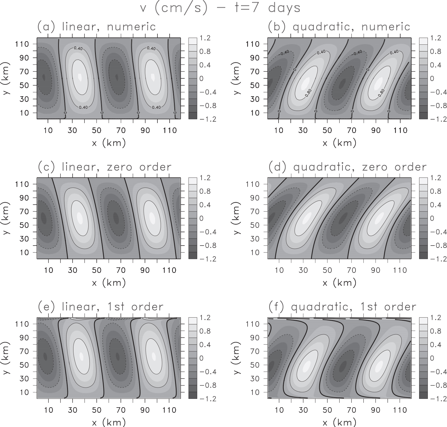
Fig. 6.
Zonal phase speed as a function of latitude for the numerical (solid), zero-order (long dashed) and first-order (short dashed) results, for the (a) linear and (b) quadratic bottom topographies. The wave propagates westward as the phase speed is negative but for the linear topography the wave propagation speed increases northwards and the opposite occurs for the quadratic topography. The phase speed calculated based on the first-order approximation is closer to the numerical one compared to the phase speed calculated based on the zero-order approximation. The phase speed was calculated based on the mean of the first 14 d of simulation.
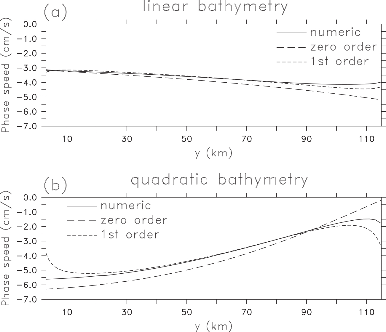
Fig. 7.
Bottom topography b(r) as a function of the radius r of the circular basin. The dashed line indicates the unperturbed free surface, H 0=90 m. This depth profile yields a constant frequency ω for the zeroth-order approximation [eq. (36)]. We choose C 1=0.
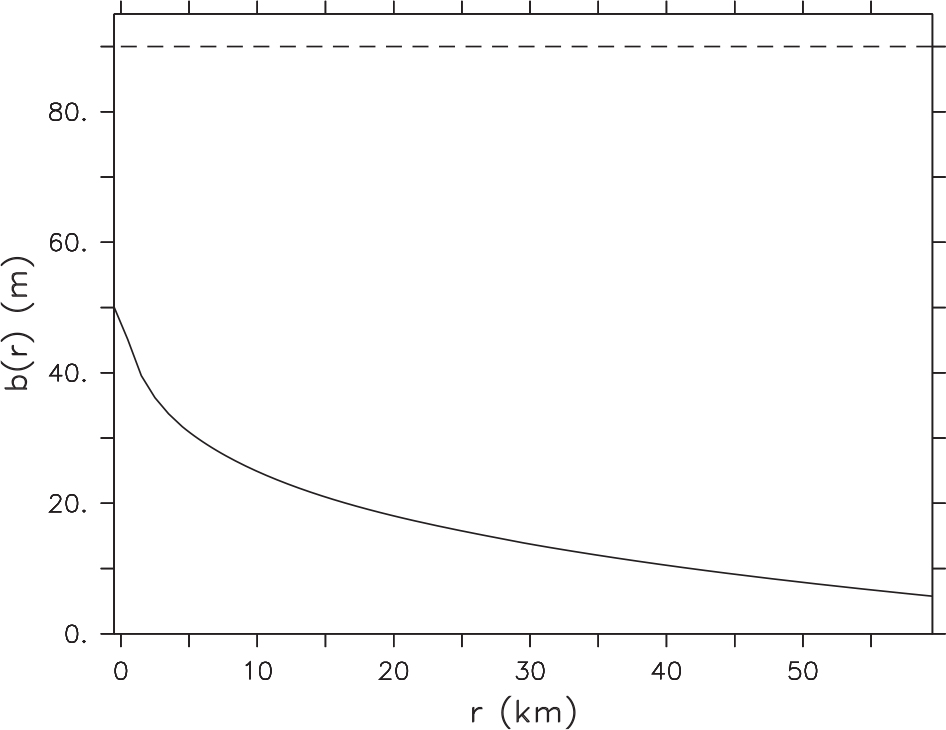
Fig. 8.
(a) Initial free surface η(θ, r). (b) The free surface of the numerical simulations for t=3 d. (c) As (b) for t=8 d. (d) As (c) but for the zero-order approximation. Note that the initial perturbation rotates clockwise and completes one full cycle in approximately 10 d. Also note that angular frequency ω(r) is almost constant as a function of radius r, as predicted by the theory.