Fig. 1.
Data assimilation experiment with the model , observations every two model steps, and M=10 and b=0.1. S-ETKF (panel a) presents EC soon after five time units while the NS-ETKF (panel b) does not. In panel (c), we quantify the clustering degree (as defined in Section 2) of the ensemble obtained for both assimilation methods as time advances.
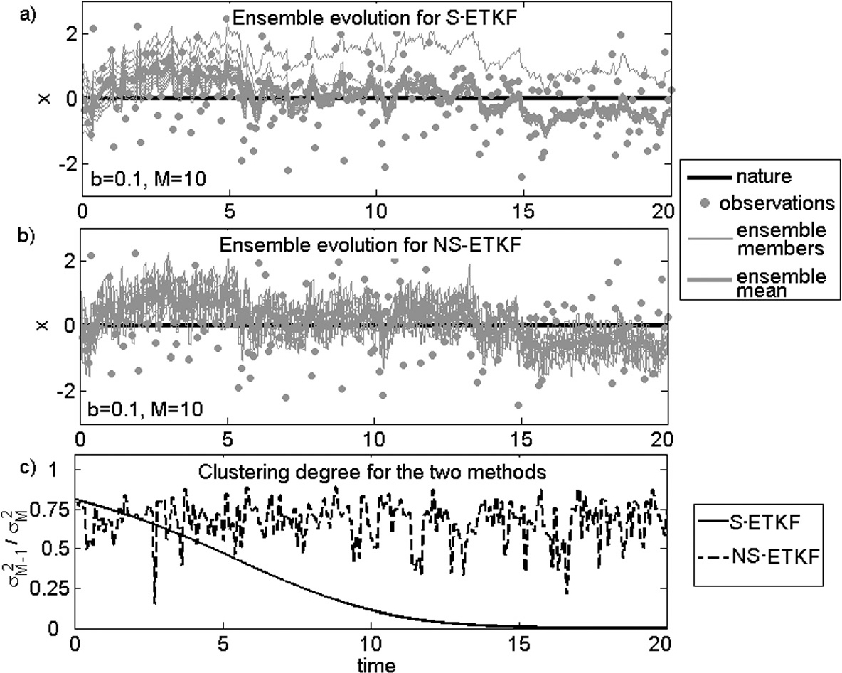
Fig. 2.
Data assimilation experiment using S-ETKF with the model and observations every two model steps. The effect of different values of non-linearity b and ensemble size M are explored. In panel (a), the time evolution of the CD metric is shown. As expected, EC appears faster as the non-linearity increases, and this appears to be independent of the ensemble size. In panel (b), we measure the time it takes for CD to get below CD c , this relationship follows a power law.
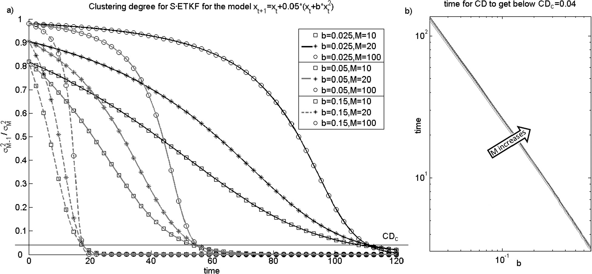
Fig. 3.
Update mechanisms for S-ETKF (panel a) and NS-ETKF (panel b) for the individual ensemble members. S-ETKF preserves the structure from the background ensemble into the analysis ensemble. The NS-ETKF effectively scrambles the ensemble every time an assimilation occurs. The model is , b=0.2, observations every five model steps, and M=10.
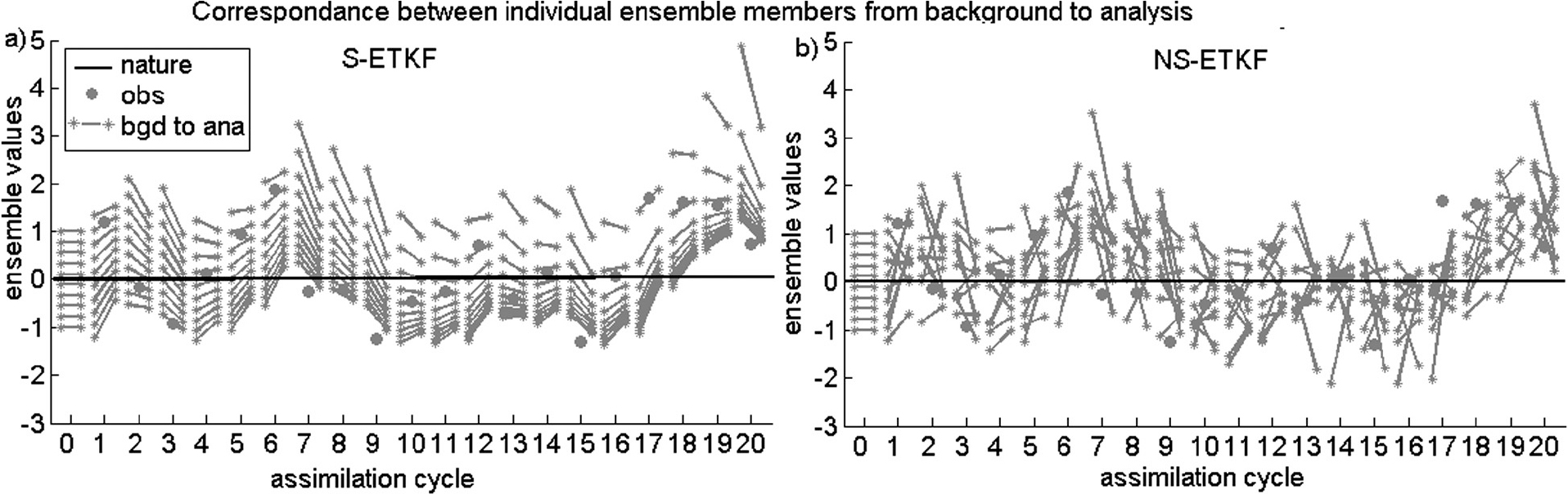
Fig. 4.
Assimilation experiments with the model . We allow the non-linear coefficient b t to vary as a piece-wise function of time (grey line, right vertical axes). CD is represented by the black line and left vertical axes. The time intervals in which b t is fixed are different for each panels: T 0=50 for (a) and T 0=500 for (b). Panel (c) shows the ensemble evolution for the time interval t∈[600, 850] of case (a); the reattachment of the outlier occurs in a natural way.
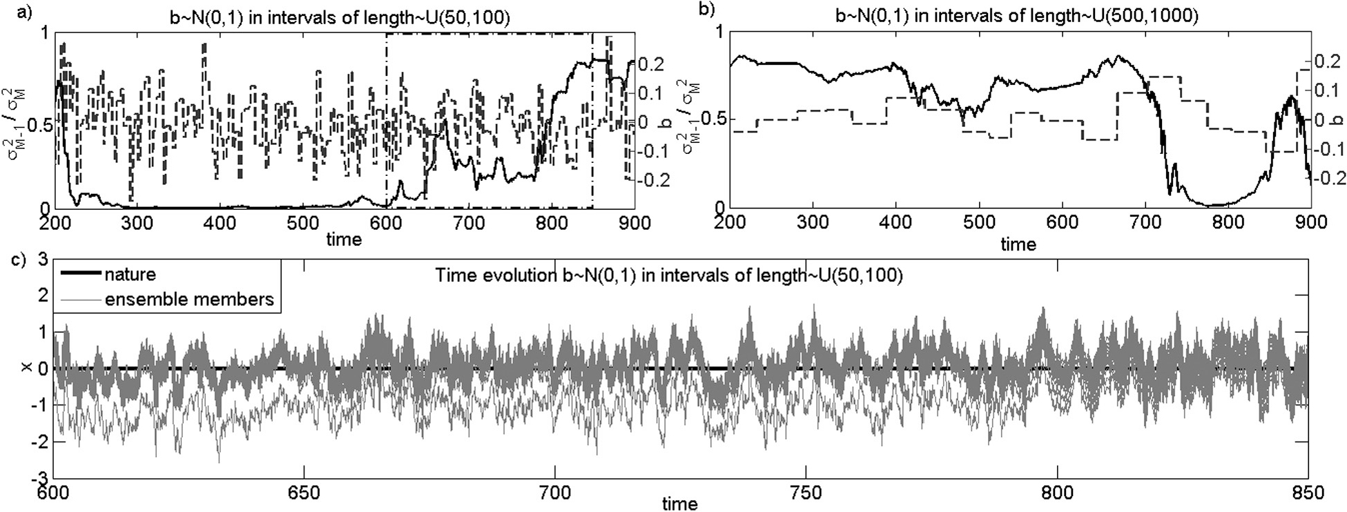
Fig. 5.
Time evolution of the CD for S-ETKF (black solid line) and NS-ETKF (grey-dashed line) from an assimilation experiment with the L63 model. Two ensemble sizes (columns) are used in a linear regime (top row) and a non-linear regime (bottom row).
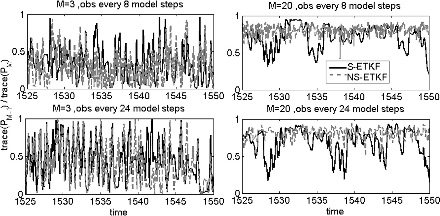
Fig. 6.
Experiments with L63, observations every 24 model steps and R=21. The evolution of the CD is shown in the top. Snapshots of the phase space are presented for three time intervals with contrasting CD values, the one in the middle shows EC occurring.
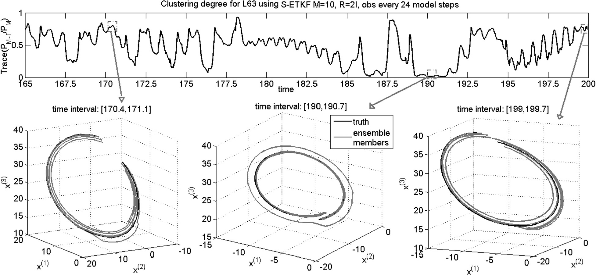
Fig. 7.
Statistical summary of the experiment with L63. In part (a), the left column shows the results in the linear regime and the right column in the non-linear regime. Boxplots for CD (top row) and analysis RMSE (bottom row) are shown for both S-ETKF and NS-ETKF. The dots inside the boxplots represent the mean for each metric; the actual values displayed. In part (b), rank histograms for the verification of the truth with respect to the analysis ensemble are presented for variable x (1).
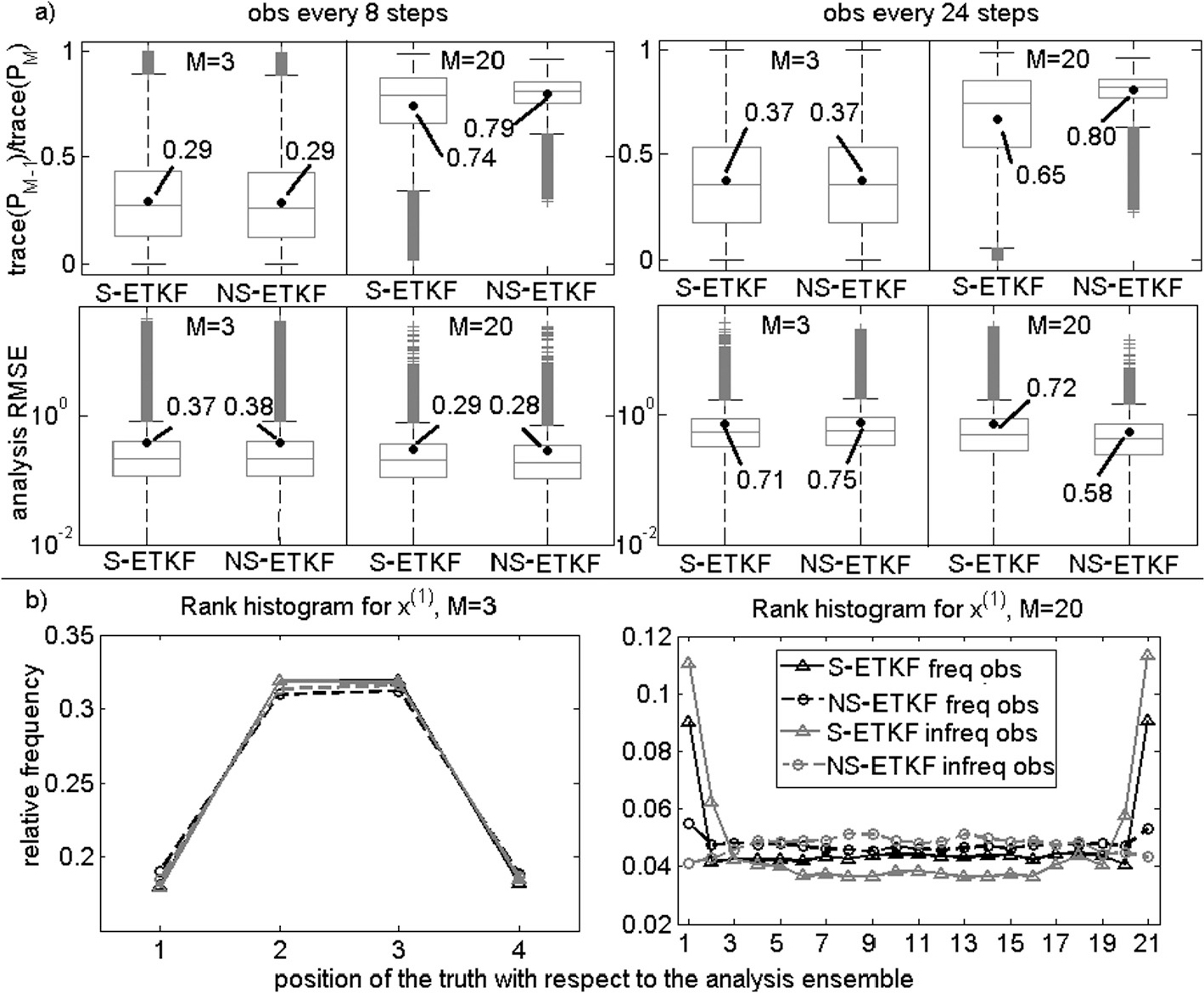
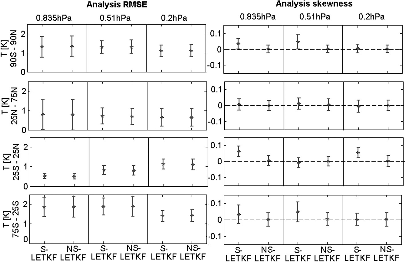
Fig. 8.
Latitude weighted analysis RMSE (left) and analysis skewness (right) for the variable T computed per region (rows) for three vertical levels (columns) in the SPEEDY model. The bars represent 1 SD of the metric around its mean. S-(L)ETKF can lead to asymmetric ensembles (e.g. in the tropics in the lower and upper atmosphere), but there is no noticeable difference in its performance with respect to NS-(L)ETKF in terms of analysis RMSE.