
Fig. 1.
The thermosyphon has a simple circular geometry. The bottom wall is heated to a constant hot temperature T h while the top wall is maintained at the temperature T c, creating a temperature inversion of hot fluid below cold fluid. If conduction alone cannot stabilise this temperature inversion, then the fluid will begin to rotate and convection becomes the dominant process of heat transfer. The relevant model state variables are proportional to the bulk fluid velocity u and the temperature difference across the loop . For CCW flow, as indicated by the arrow near 9 o'clock, fluid velocity and is typically >0. The radius ratio used in our experiments is shown to scale.
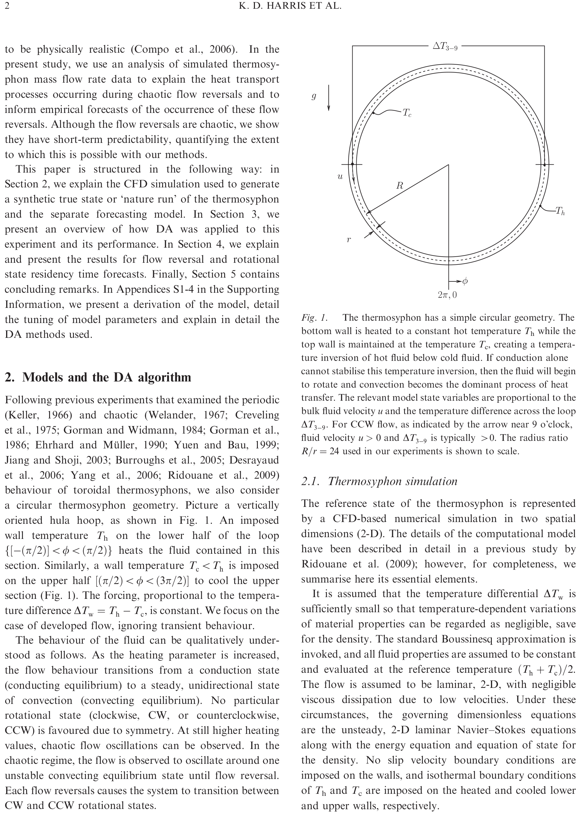
Fig. 2.
An illustration of the basic predict-observe-update DA cycle. The EM model states (background forecast and analysis) are transformed into observations of the mass flow rate q by the observation operator [eq. (4)] for comparison with the truth. Here, using the 3-D-Var algorithm and an assimilation window of 5 min, the filter has satisfactory overall performance (scaled error≈35%). Note the error spike around 135 min when the forecast and truth end up in different rotational states. The largest errors tend to occur at or near flow reversals due to inherent sensitivity near that transition and to the qualitatively different behaviour of the different flow directions.
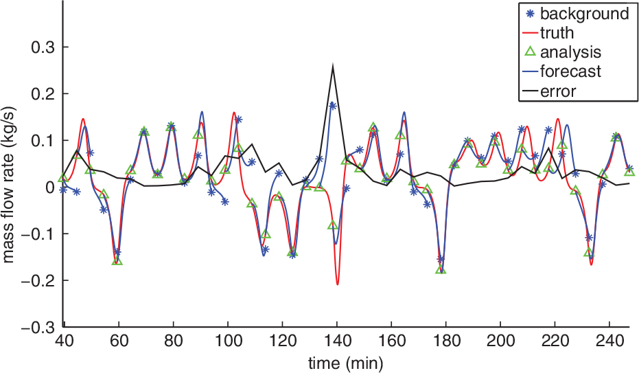
Fig. 3.
Background RMSE scaled by over 2500 assimilation cycles plotted for different DA algorithms and varying assimilation windows. As the window becomes larger, the error increases towards saturation. The lower dashed line in the main figure shows the limit of a ‘perfect’ forecast while the upper demarcates a ‘useless’ forecast.
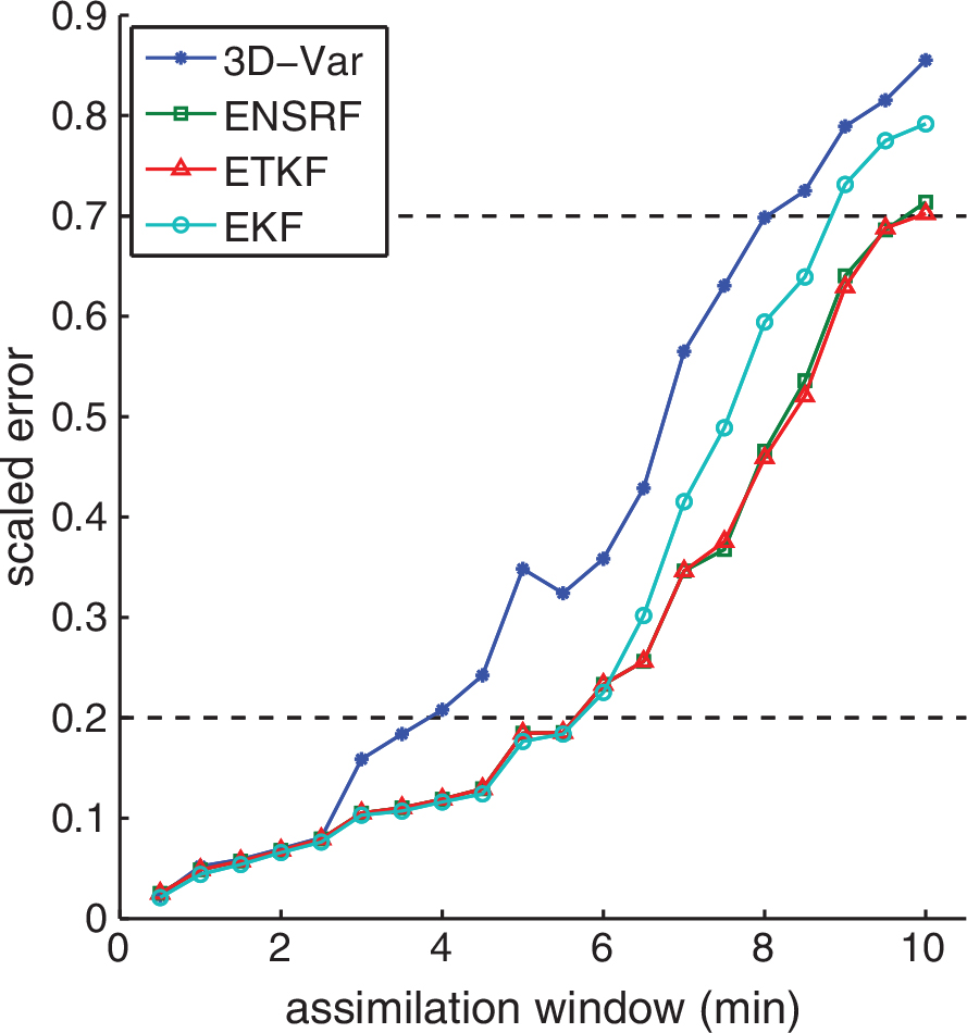
Fig. 4.
Two views of the numerically simulated thermosyphon attractor. A time-delay reconstruction, using the monitored mass flow rate, is shown in (a). In (b), plotted points show x 1 and x 2 of the EM analysis generated by EKF with an assimilation window of 120 s. Each is coloured by the scaled background forecast error at that point. The delay time of 60 s used for (a) was chosen because it yielded a good approximation of the attractor in (b). Note how in (a) trajectories that move through the far edge of either lobe create distinctive loops near the centre of the opposite lobe. This is an example of dynamics which are not present in the EM model without DA. It may explain the higher error for points in (b) at the far edge of each attractor lobe. See text for further description and Fig. 5 for another example.
Fig. 5.
The assimilated trajectory during a very large oscillation, non-Lorenz flow reversal. The EKF algorithm with a 30 s assimilation window was used. Colour indicates the scaled background error. The state starts (a) in the CCW rotational region and stalls near the conducting state for an extended period, causing fluid in the bottom to heat up, manifesting in an x 3 that creeps towards 0 with x 1, x 2≈0, before the state swings quickly (b) through one oscillation in the CW rotational state. This is followed by one oscillation in the CCW state (c) before another stall near the conducting point and subsequent swing (b again) before settling into Lorenz-like oscillations (d). Note that the filter only observes the x 1 variable but is able to reconstruct the dynamics in the full state space.
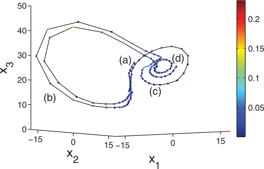
Fig. 6.
Correlation test: whenever the slope (green) of the correlation exceeds a threshold (red), a flow reversal is forecast. Correct positive predictions are shown as filled circles and false positives as open circles. The starred point corresponds to the inset, which shows how correlation is computed as the slope of the least squares fit (green line) of previous analysis points, and the arrow shows the direction of the trajectory. Note that each analysis cycle where the correlation fails to exceed the threshold counts as a correct negative forecast (not shown). There are no false negatives, that is misses, in this timeseries. Here, and are the same as for Table 1.
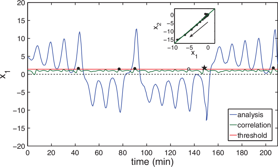
Fig. 7.
Residency time in the new rotational state is plotted versus the amplitude of x 1 (proportional to the mass flow rate) at the last extremum before flow reversal. This amplitude is calculated from the EM model EKF analysis of thermosyphon observations, using a 30 s assimilation window. This figure contains over 39 d of simulated flow and 1796 flow reversals. Points are coloured by the average BV growth rate over the preceding assimilation window, showing a BV growth rate gradient that increases in the positive direction along both axes. Inset, upper left: a timeseries corresponding to a single point in the scatter plot, marked with a black cross. The x 1 oscillation amplitude and subsequent residency time are denoted by the vertical and horizontal arrows, respectively. Inset, upper right: a histogram showing the likelihood of residency times following an . This is the interval that we would consider for an x 1 oscillation amplitude of 10.5 preceding flow reversal. The most likely residency time is about 23 min or two oscillations, the middle ‘step’ for the histogram range.
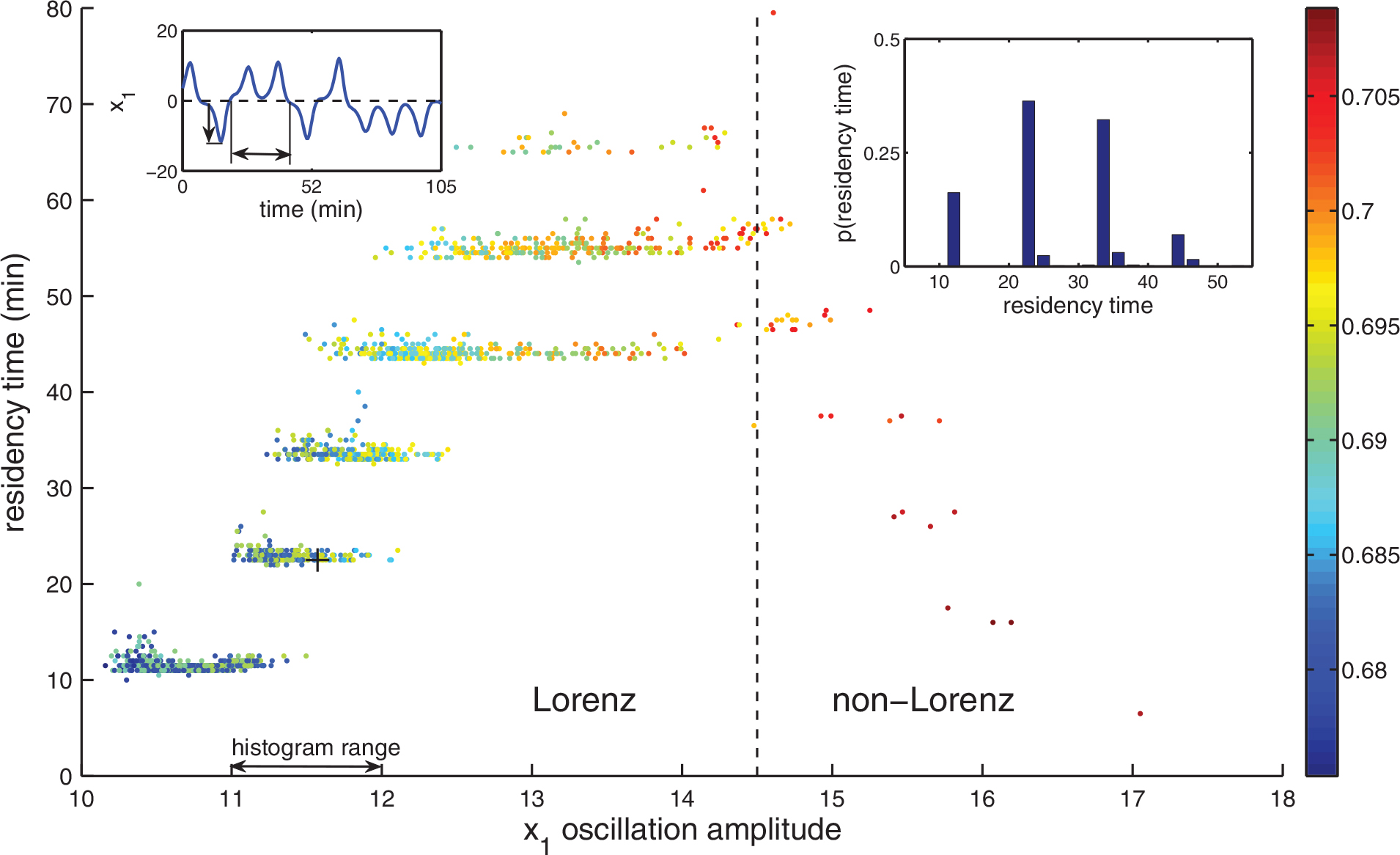
Fig. 8.
Temperature profiles before and after two flow reversals for the chaotic regime in units of Kelvin. For ease of visualisation, the radius ratio is reduced to 3 (). The amplitude of the oscillation shown in (a) is relatively weak; the temperature profile quickly approaches (b) that of conduction (c) where it heats up significantly before the reversal. The extreme instability of the conducting state, near time 20 min, produces a large oscillation in the CW direction (d), immediately causing another flow reversal back to CCW. As the system enters the new rotational state, remnant heat stabilises the flow [contrast (e − f) with (b − c)], necessitating a longer residency in the new rotational state while the instability grows (g − i) (note that for the radius ratio of 24 no more than seven oscillations are ever observed).
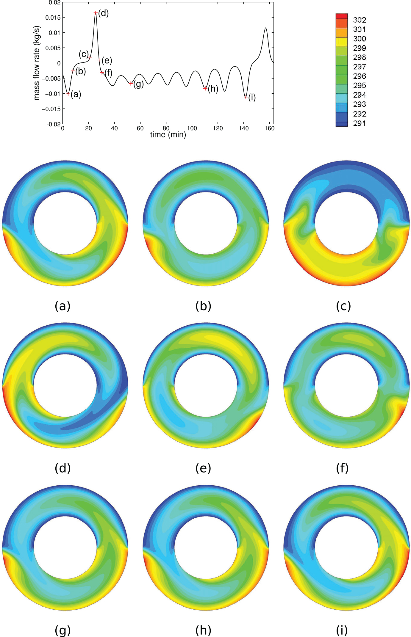
Table 1. Contingency tables for the three flow reversal tests
[i] The parameters used were: , , and . For a detailed description of the tuning, see the text and Fig. S3-2 in Appendix S3 in the Supporting Information.
Table 2. Skill scores for flow reversal categorical forecasts (TS, FAR and POD) and residency time probabilistic forecasts (RPS-avg and RPS-med) for the three tests
[i] Note that for TS and POD, a perfect score is 100% while a perfect FAR is 0%; RPS scores should be interpreted as a percent improvement over climatology, so that any RPS > 0 is an improvement.