
Fig. 1.
Standard deviations of differences between vorticity forecasts valid at the same time (dotted lines) and SDs of differences between 5-h vorticity forecast tendencies valid at the same time (full lines), both given as functions of the vertical level.
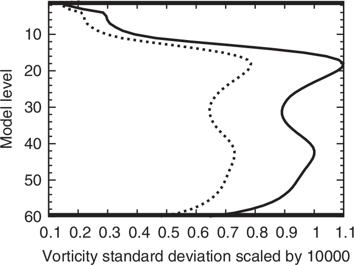
Fig. 2.
Horizontal variance spectra normalised with the total variance for differences between vorticity forecasts valid at the same time (thin lines) and for differences between 5-h vorticity tendencies valid at the same time (thick lines). Model level 30 (500 hPa, full lines) and model level 50 (850 hPa, dotted lines).
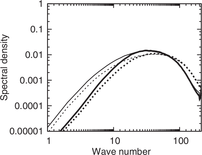
Fig. 3.
Time correlation of vorticity forecast differences at model level 30 (500 hPa, full line) and model level 50 (850 hPa, dotted line).
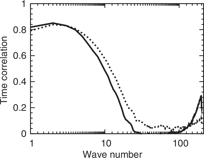
Fig. 4.
The model level 15 (300 hPa) wind background field, 3 December 1999 00UTC +6 h, applied during the single observation impact experiments. The contour interval is 10 m s−1.
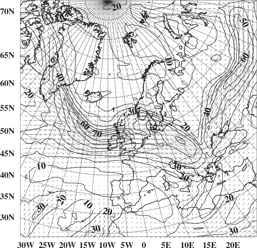
Fig. 5.
Model level 15 wind field assimilation increments from a simulated south-westerly wind observation increment of 9 m s−1 at 3 December 1999 11UTC in the position 32°N, 12°W (marked OBS). With control of lateral boundary conditions (method lbc1). 3 December 1999 06 UTC (upper), 09 UTC (middle) and 11 UTC (lower). The contour interval is 1 m s−1.
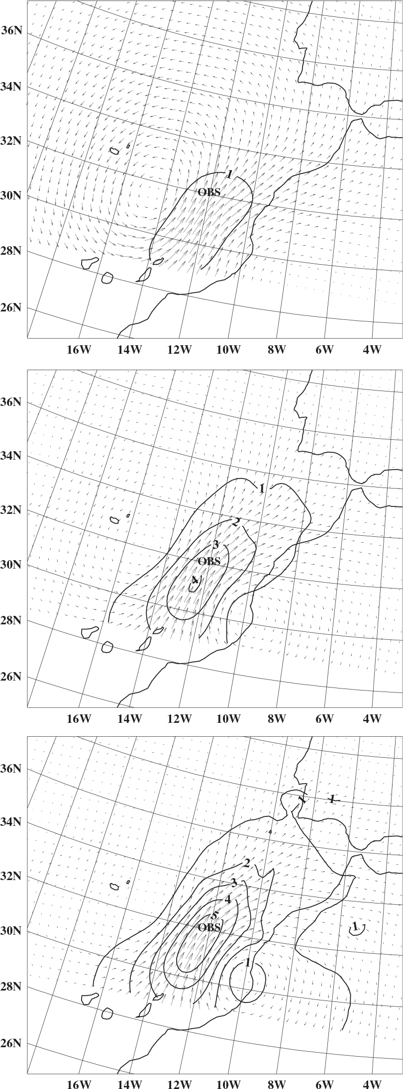
Fig. 6.
Model level 15 wind field assimilation increment at 3 December 1999 09 UTC from a simulated south-westerly wind observation increment of 9 m s−1 at 3 December 1999 11UTC in the position 32°N, 12°W (marked OBS), without control of lateral boundary conditions. Zero-valued lateral boundary conditions at the initial time (method nolbc1, upper), lateral boundary conditions at the initial time equal to the initial condition increments (method nolbc2, lower). The contour interval is 1 m s−1.
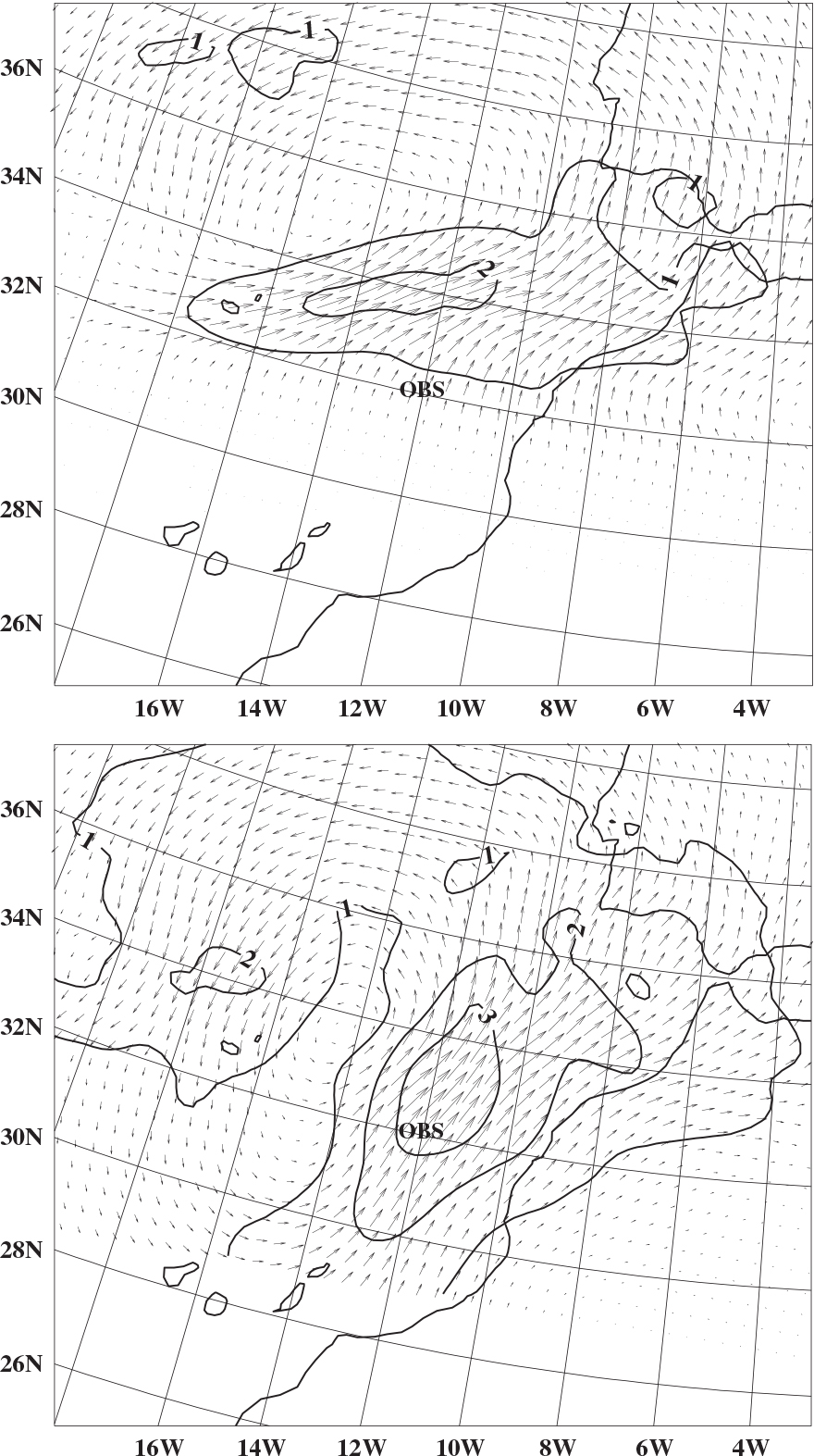
Fig. 7.
The SMHI 11 km data assimilation and forecast domain.
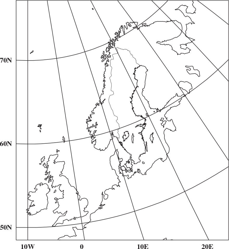
Fig. 8.
BIAS (mean error) and SD (standard deviation of error) verification scores for mean sea level pressure forecasts over a Scandinavian domain as verified against SYNOP observations for the forecast lengths +0 h, +6 h, +12 h, +18 h, +24 h, +30 h and +36 h. Verification scores are averaged for the month of December 1999. Experiments nolbc1 (red lines), nolbc2 (green lines), lbc1 (blue lines) and lbc2 (pink lines). Grey line marked CASES shows the number of verifying observations.
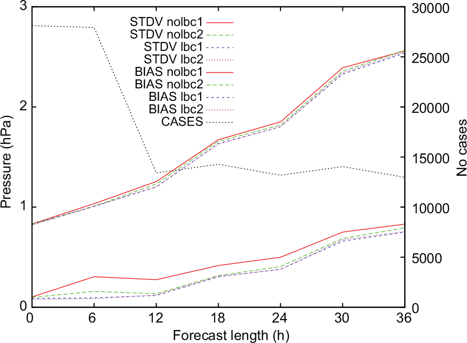
Fig. 9.
BIAS (mean error) and SD (standard deviation of error) verification scores for relative humidity profile forecasts over a European domain as verified against radiosonde observations at 12 UTC. Verification scores are averaged for the month of December 1999 and for +12 h, +24 h and +36 h forecasts. Experiments nolbc1 (red lines), nolbc2 (green lines), lbc1 (blue lines) and lbc2 (pink lines). Grey line marked CASES shows the number of verifying observations. The EWGLAM (European Working Group on Limited Area Models) list of verifying radiosonde stations is applied.
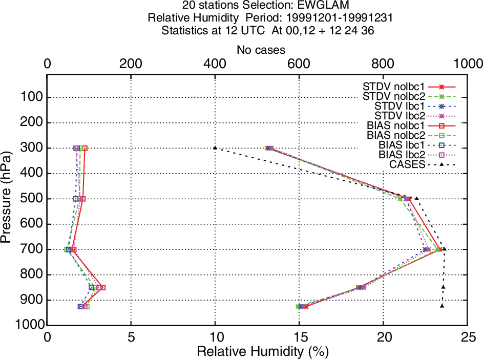
Fig. 10.
BIAS (mean error) and SD (standard deviation of error) verification scores for 500 hPa temperature forecasts over an European domain as verified against radiosonde observations for the forecast lengths +0 h, +12 h, +24 h and +36 h. Verification scores are averaged for the month of December 1999. Experiments nolbc1 (red lines), nolbc2 (green lines), lbc1 (blue lines) and lbc2 (pink lines). Grey line marked CASES shows the number of verifying observations. The EWGLAM (European Working Group on Limited Area Models) list of verifying radiosonde stations is applied.
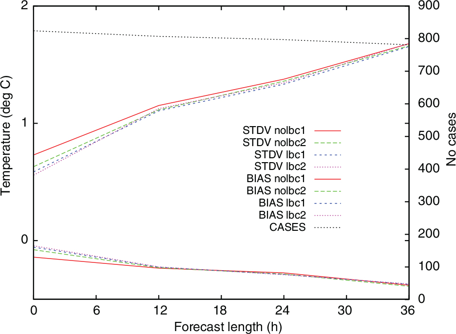
Fig. 11.
BIAS (mean error) and SD (standard deviation of error) verification scores for 500 hPa temperature forecasts over a Scandinavian domain as verified against radiosonde observations for the forecast lengths +0 h, +12 h, +24 h and +36 h. Verification scores are averaged for the month of December 1999. Experiments nolbc1 (red lines), nolbc2 (green lines), lbc1 (blue lines) and lbc2 (pink lines). Grey line marked CASES shows the number of verifying observations.
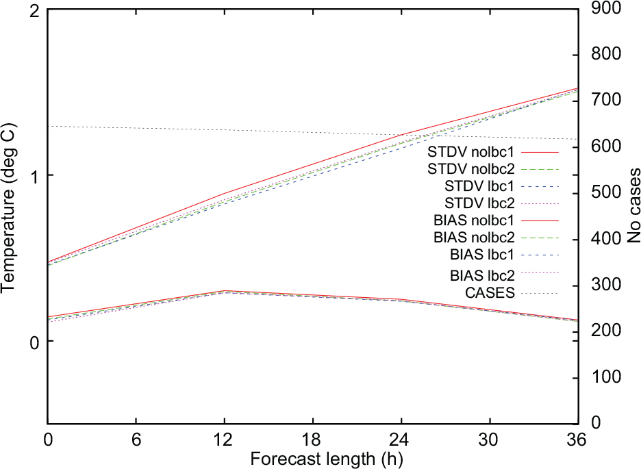
Fig. 12.
Mean sea level pressure forecasts 5 December 1999 00UTC + 36 h over a Nordic area without control of lateral boundary conditions (experiment nolbc1, left) and with control of lateral boundary conditions (experiment lbc1, middle). Mean sea level pressure analysis 6 December 1999 12 UTC (experiment lbc1, right). The contour interval is 2 hPa.
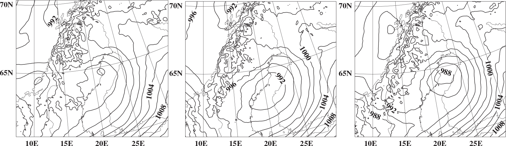
Fig. 13.
Differences between surface pressure forecasts, forecasts utilising control of lateral boundary conditions (experiment lbc1) minus forecast not using control of lateral boundary conditions (experiment nolbc1), 5 December 00 UTC +36 h (upper left), +24 h (upper right), +12 h (lower, left) and +00 h (lower, right). The contour interval is 1 hPa.
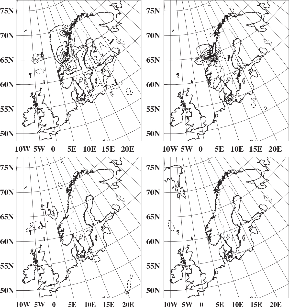
Fig. 14.
Adjoint model sensitivities of the +36 h forecast differences in Fig. 12 (upper, left) with regard to the initial model level 20 (500 hPa) temperatures (left) and with regard to initial and initial lateral boundary conditions model level 20 temperatures (right). The contour interval is 2 K.
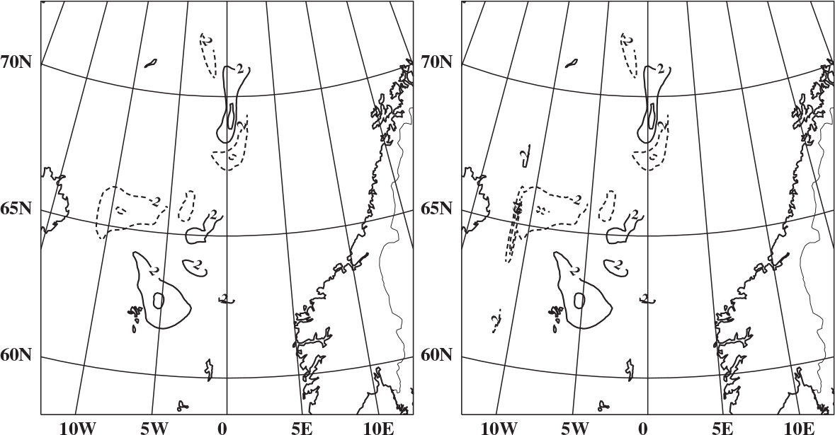
Table 1. Average number of conjugate gradient iterations, maximum number of conjugate gradient iterations, average computing time and maximum computing time for 4D-Var minimisations over December 1999
[i] Two versions of handling the control of lateral boundary conditions and two versions without control of lateral boundary conditions are compared.