Table 1. Parameters of the sea ice scheme used in GME and COSMO
Fig. 1.
Lake surface temperature θ sfc (θ f0=273.15 K is the fresh-water freezing point) in Neusiedlersee over the period from 1 January to 30 April 2006. Blue curve shows the lake surface temperature predicted by FLake (00 UTC values from the assimilation cycle), and red curve shows the temperature from the routine COSMO SST analysis (performed once a day at 00 UTC). Curves are the results of averaging over the COSMO-model grid boxes that constitute the lake in question. An asterisk shows the observed time of lake-ice break-up.
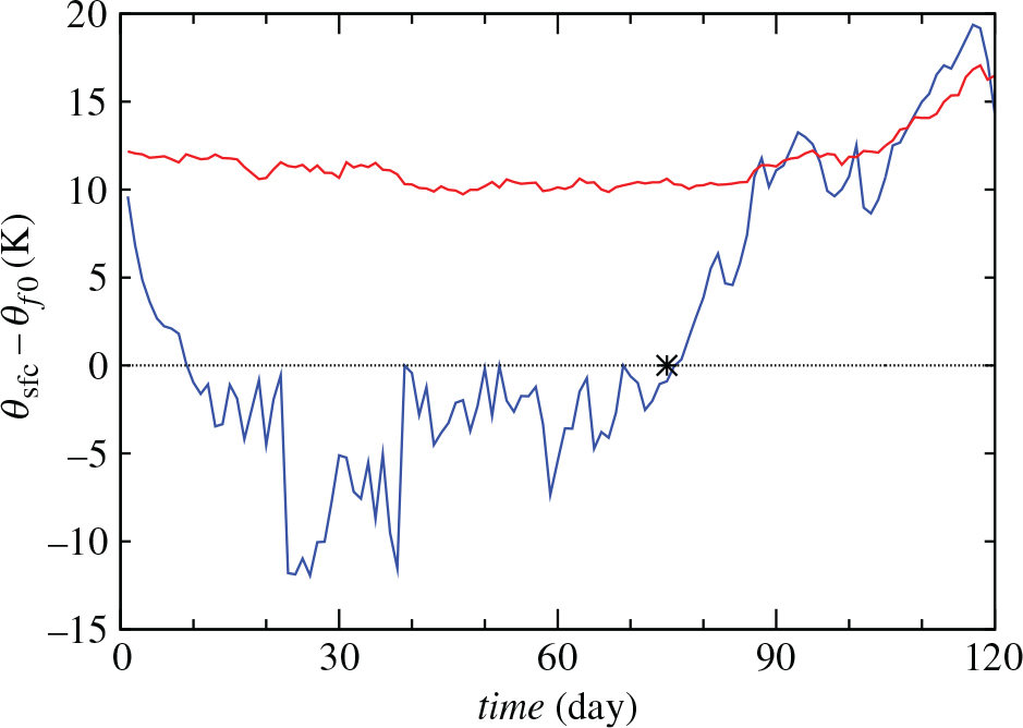
Fig. 2.
The same as in Fig. 1 but for Lake Sniardwy.
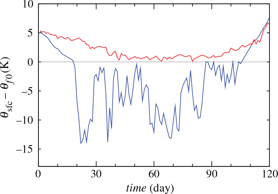
Fig. 3.
Bias of the two-metre temperature (T2m) vs. forecas time for the period from 3 to 28 February 2010. Lines show the COSMO-EU forecasts initialised at 00 UTC: blue line – with the sea-ice scheme, and red line – without the sea-ice scheme. Observational data used for verification are from the land meteorological stations in the neighbourhood of the Baltic Sea (see text for further explanations).
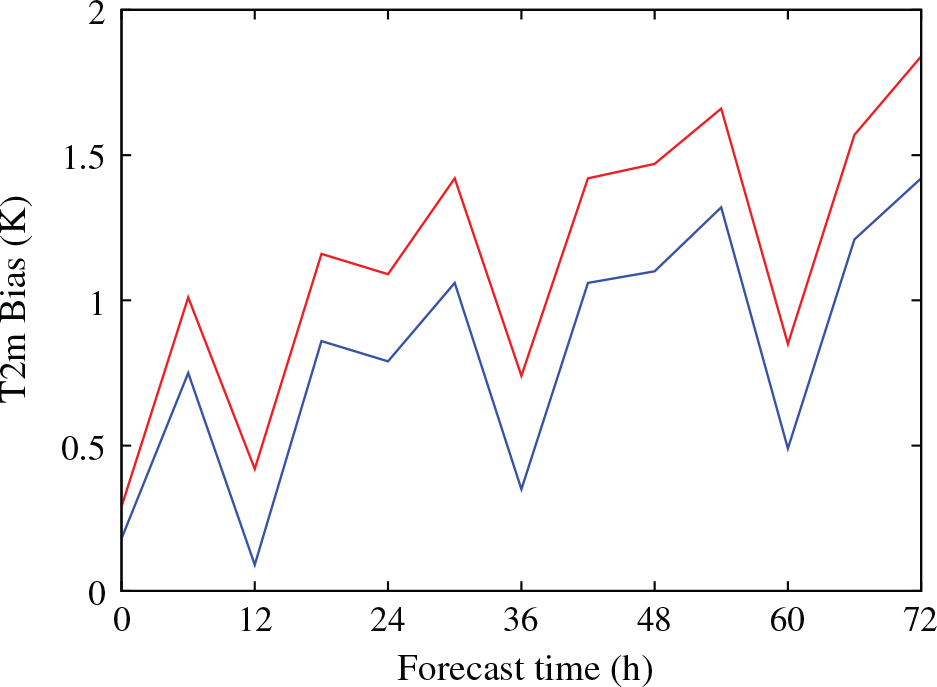
Fig. 4.
The same as in Fig. 3 but for the two-metre temperature r.m.s.e.
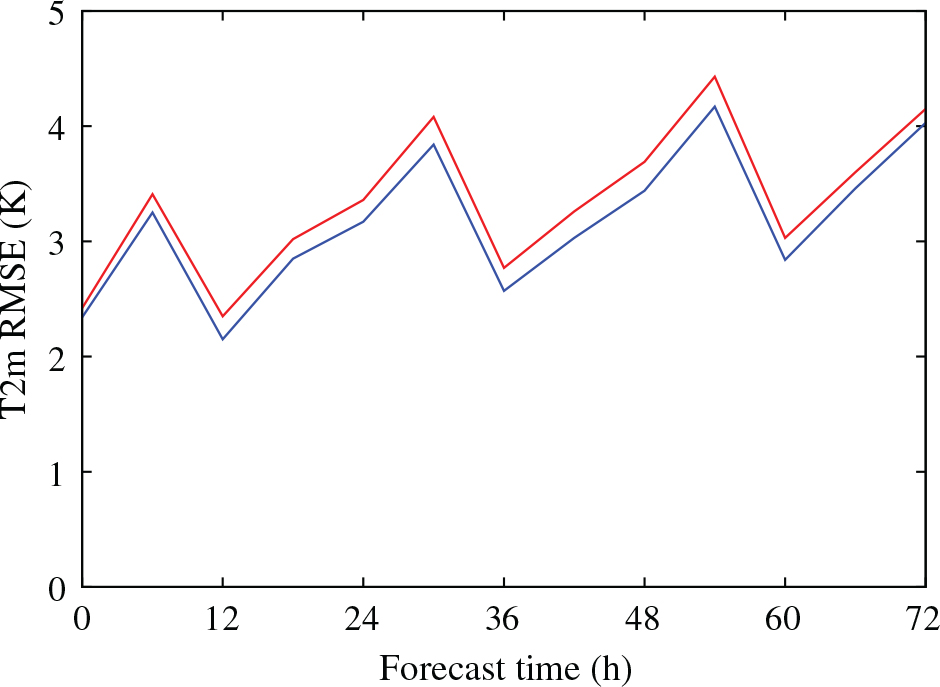
Fig. 5.
The two-metre temperature bias in the Arctic at 12 UTC 1 January 2004: left panel – GME analysis using the old ice scheme, right panel – GME analysis using the ice scheme described in the present paper. Numbers show computed minus observed two-metre temperature difference (K).
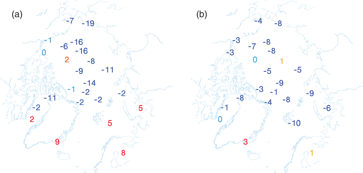
Fig. 6.
The grid-box mean surface temperature θ g in the Arctic over the period from 30 January 2009 to 19 January 2011. Curves show the 24 h forecasts initialised at 00 UTC: blue curve – GME, and red curve – ECMWF. The curves are computed by means of averaging over all sea-ice points north of 65 N latitude using the GME ice-water mask.
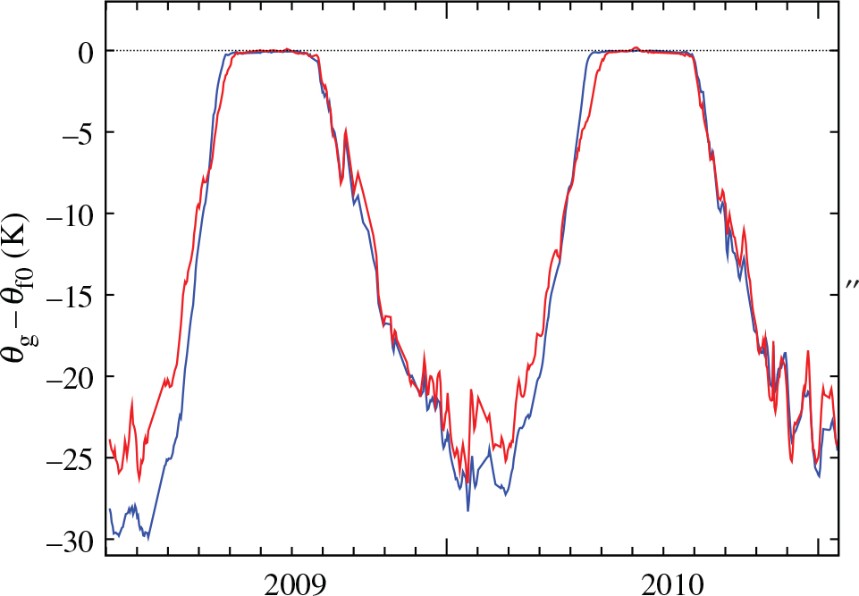
Fig. 7.
The net surface long-wave radiation flux Q lw (positive downward) in the Arctic over the period from 30 January 2009 to 19 January 2011. Curves show values averaged over the first 24 hours of the forecast initialised at 00 UTC: blue curve – GME, and red curve – ECMWF. The curves are computed by means of averaging over all sea-ice points north of 65 N latitude using the GME ice-water mask.
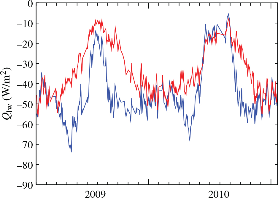
Fig. 8.
The same as in Fig. 7 but for the net surface flux of solar radiation Q sol (positive downward).
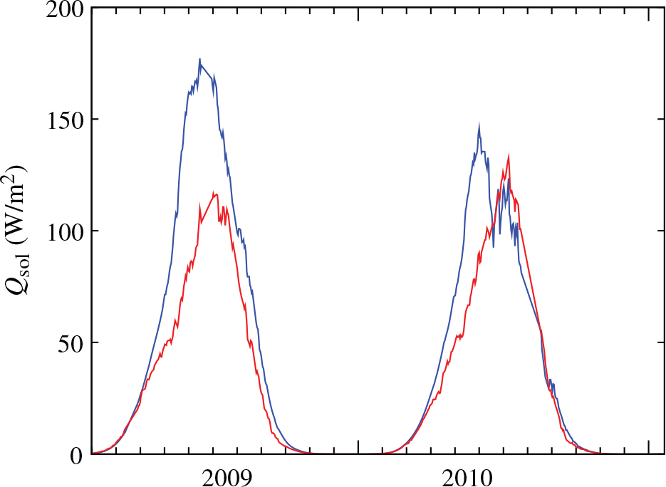
Fig. 9.
Ice thickness in Lake Pääjärvi during winter 1999–2000, where day=0 corresponds to 1 January 2000. Blue curves show results of simulations with FLake: solid curve – with a snow layer above the ice, and dashed curve – no snow above the ice. Red symbols show observational data.
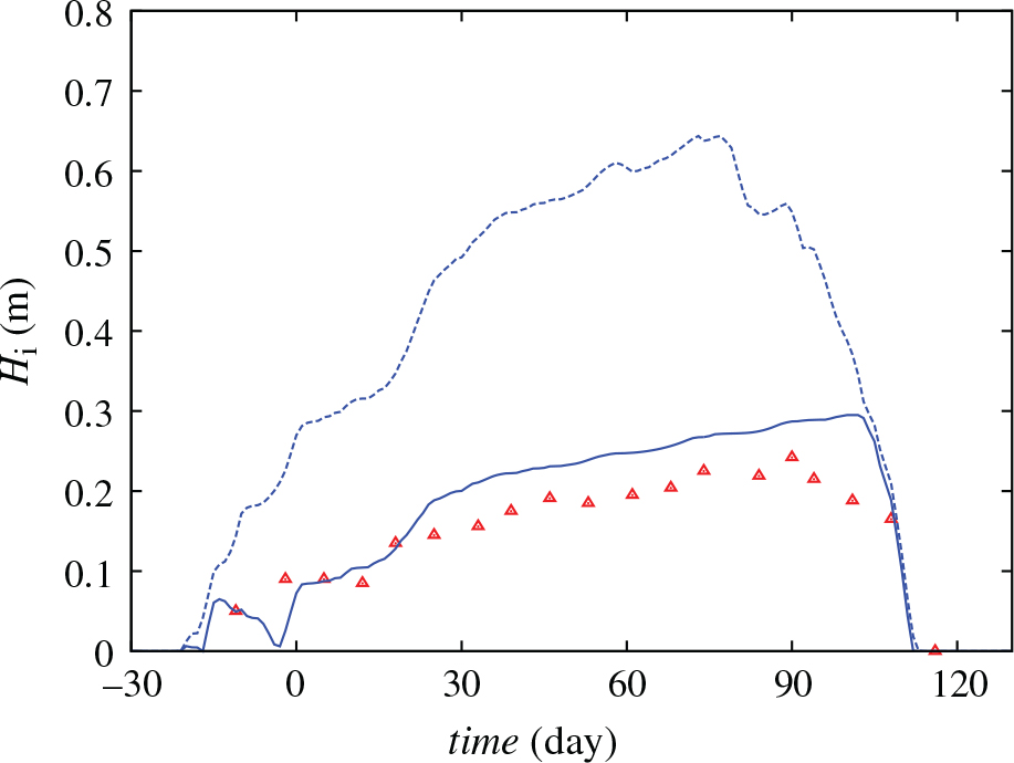
Fig. 10.
Snow thickness in Lake Pääjärvi during winter 1999–2000, where day=0 corresponds to 1 January 2000. Blue curve is computed with FLake. Black solid and dashes curves show observed values of the snow thickness and the snow ice thickness, respectively. Red curve with symbols shows the total thickness of the two layers.
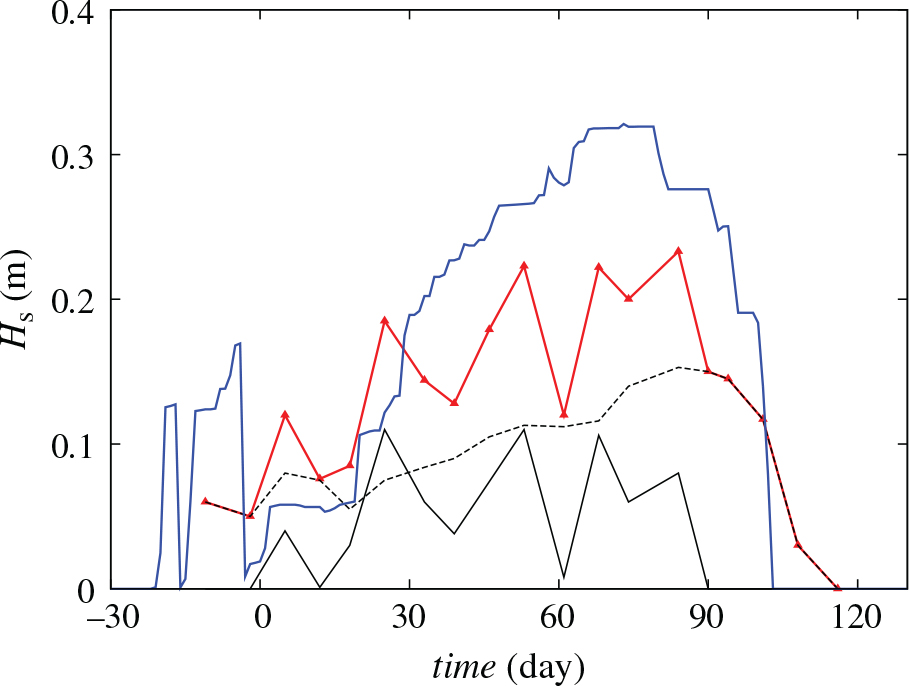
Fig. 11.
Surface temperature of Lake Pääjärvi during winter 1999–2000, where day=0 corresponds to 1 January 2000. The lake surface temperature is equal to the surface temperature of snow, ice or water depending on which surface is exposed to the atmosphere (snow, ice or open water). Blue solid and dashed curves show results of simulations with and without a snow layer above the ice, respectively. Red curve shows observed water surface temperature.
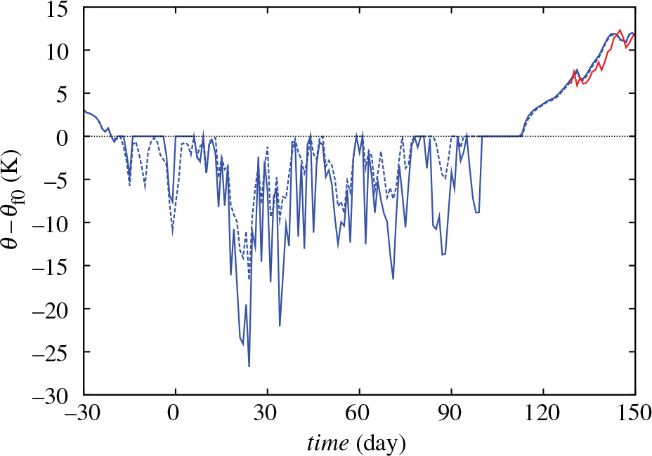
Fig. 12.
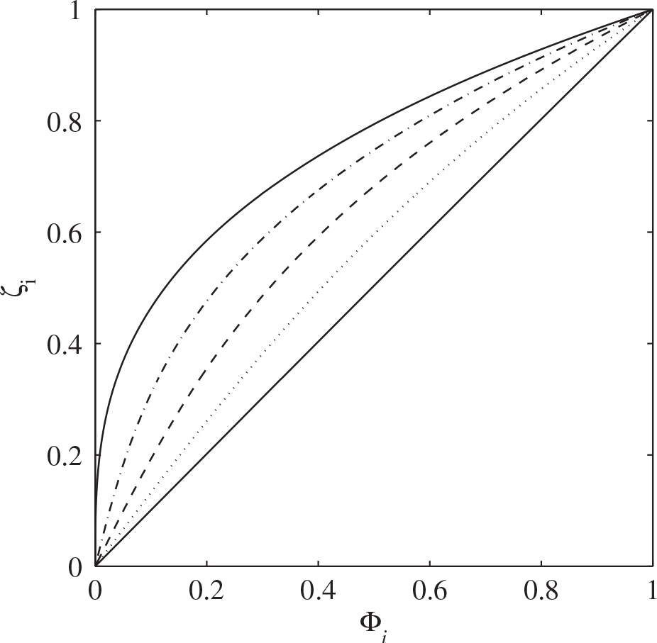
The approximation of the temperature-profile shape function with the third-order polynomial whose coefficients satisfy Eq. (B.1). The curves are computed with and (from right to left) , , , , and .