
Fig. 1.
Geographical location of Lake Vanajavesi (A); surrounding observation sites Jokioinen meteorological observatory (B), Lake Kuivajärvi (C) and Lake Pääjärvi (D).
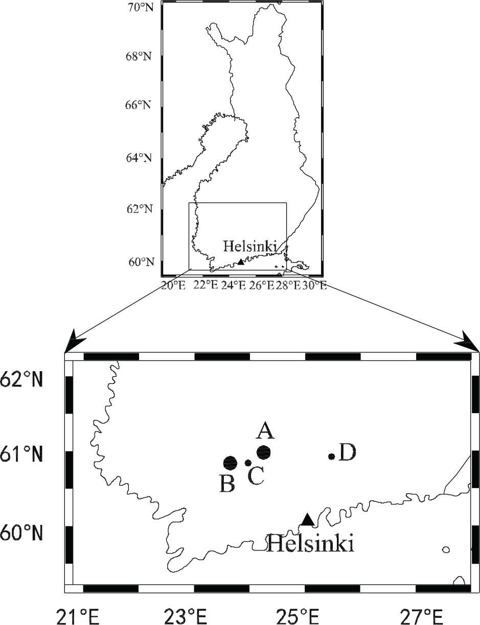
Fig. 2.
Time series of wind speed (a), air temperature (b), relative humidity (c), cloudiness (d) and precipitation (e). The data were initially observed at 3-hour time interval.
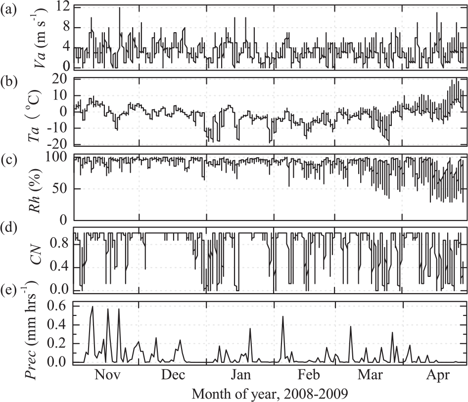
Table 1. The monthly mean meteorological data for 1971–2000 (Drebs et al., 2002; h′ s is snow thickness on the 15th of each month; Ph s is the portion of precipitation contributing to the snow accumulation)
Table 2. Model parameters found in the literature
Fig. 3.
Time series of observed and modelled snow and ice thickness. The dark grey line and the asterisk are the observed snow thickness in Jokioinen and on Lake Vanajavesi, respectively. The black dashed and solid lines are modelled snow and ice thickness (reference experiment), respectively. The circles are the observed average ice thickness, and the spatial standard deviation is indicated by the vertical bar.
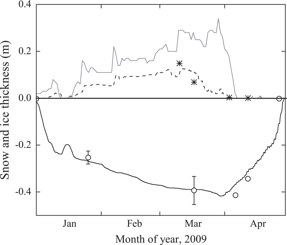
Fig. 4.
Time series of observed and simulated ice thickness based on varying heat flux from water: 0 W m−2 (black dashed), 0.5 W m−2 (black solid; reference experiment), 2 W m−2 (grey dashed) and 5 W m−2 (grey solid). Measurements of ice thickness are shown as in Fig. 3.
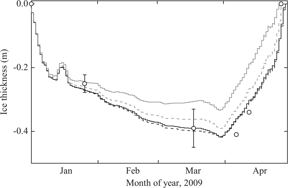
Fig. 5.
Calculated and observed incoming short-wave radiative flux under clear and cloudy sky conditions. The data cover the winter 2008–2009 from January to April. Goodness of fit for the whole ice season's data was R 2=0.92 (n=2880).
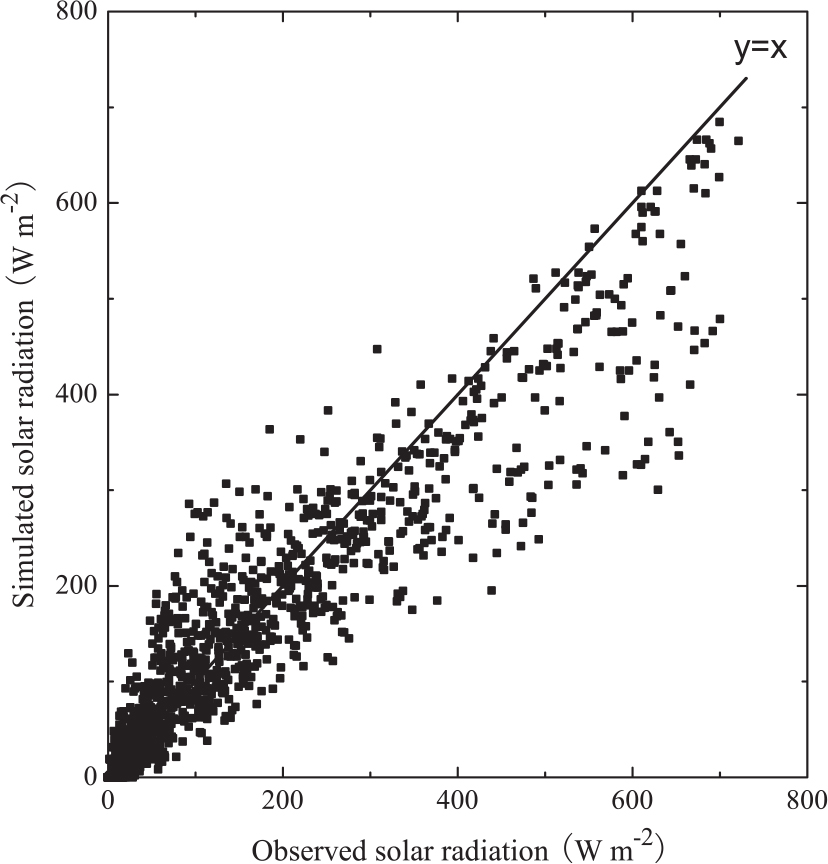
Fig. 6.
Surface temperature versus ice thickness: for a cold period 0000 hr 3 January through 2300 hr 5 January (a); for a warm period 0000 hr 8 April through 1300 hr 11 April (b). In both cases, the snow was set to be zero for simplicity.
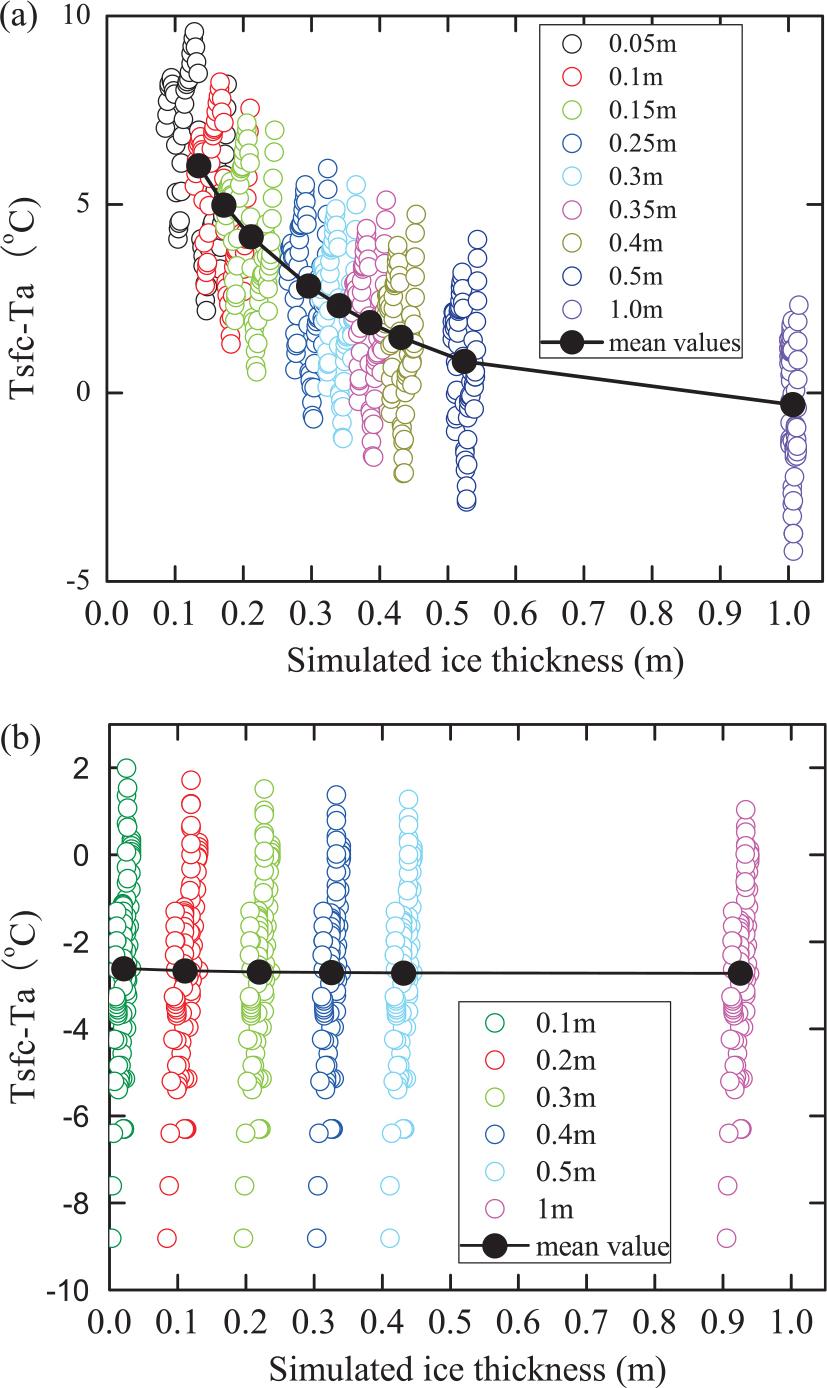
Fig. 7.
Time series of simulated snow (grey line) and ice (black line) thickness. The circles show the mean ice thickness observed in the middle of each month in Lake Kuivajärvi (60.76°N, 23.88°E; cf. Fig. 1) located southwest (60 km) from Lake Vanajavesi.
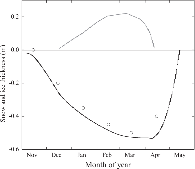
Table 3. Initial setup (T a, h s, h i) for 10-d simulations and simulated ice growth rate (dh i/dt)
Fig. 8.
Ten-day modelled ice thickness based on air temperature varying sinusoidally (red lines) and constant mean values (black lines) for each winter month: November (a); December (b); January (c); February (d); March (e) and April (f).
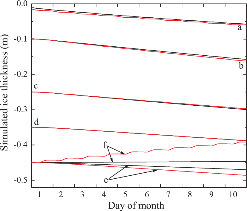
Fig. 9.
Model sensitivity to the air temperature. The black solid line is the reference of present climate. The grey solid (dashed) line and light grey solid (dashed) line are modelled ice thickness based on air temperature decreasing (increasing) 5 and 1°C, respectively.
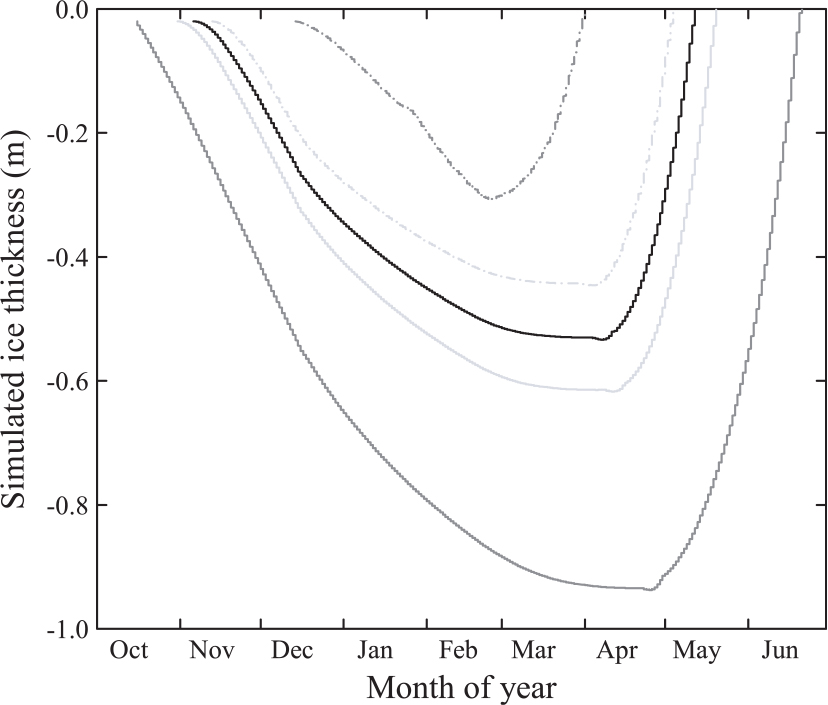
Table 4. The daily mean heat fluxes contributing to the surface heat balance (W m−2). The columns are surface layer absorption of solar radiation, net longwave radiation, sensible heat flux, latent heat flux, conductive heat flux from below and heat flux for melting