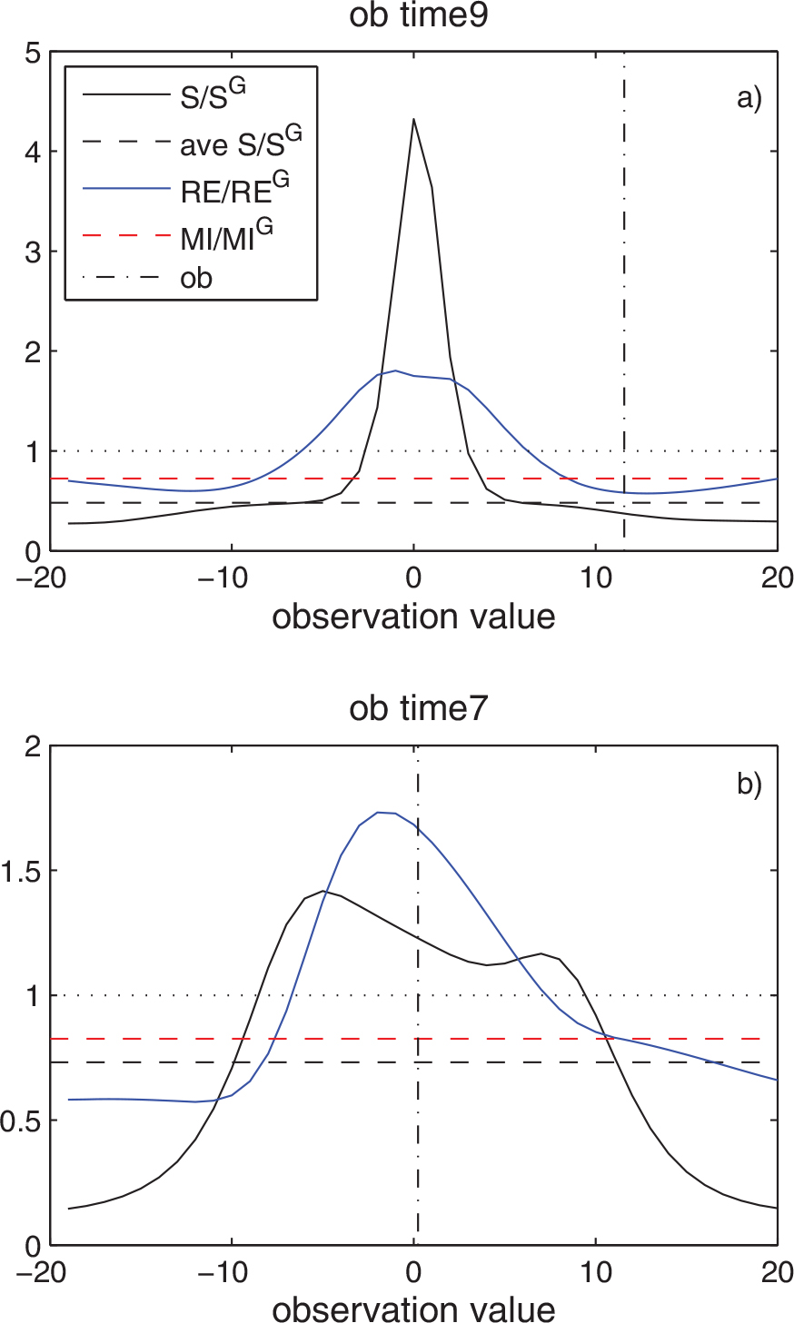
Fig. 1.
Left: the prior distribution. The vertical blue line shows the prior mean, µ x . Right: (solid) and the Gaussian approximation (dashed) for k=2, σ 2=1, w=0.25, µ 1=−1.5, µ 2=−1.5. µ −, µ 0 and µ + explained within the text.
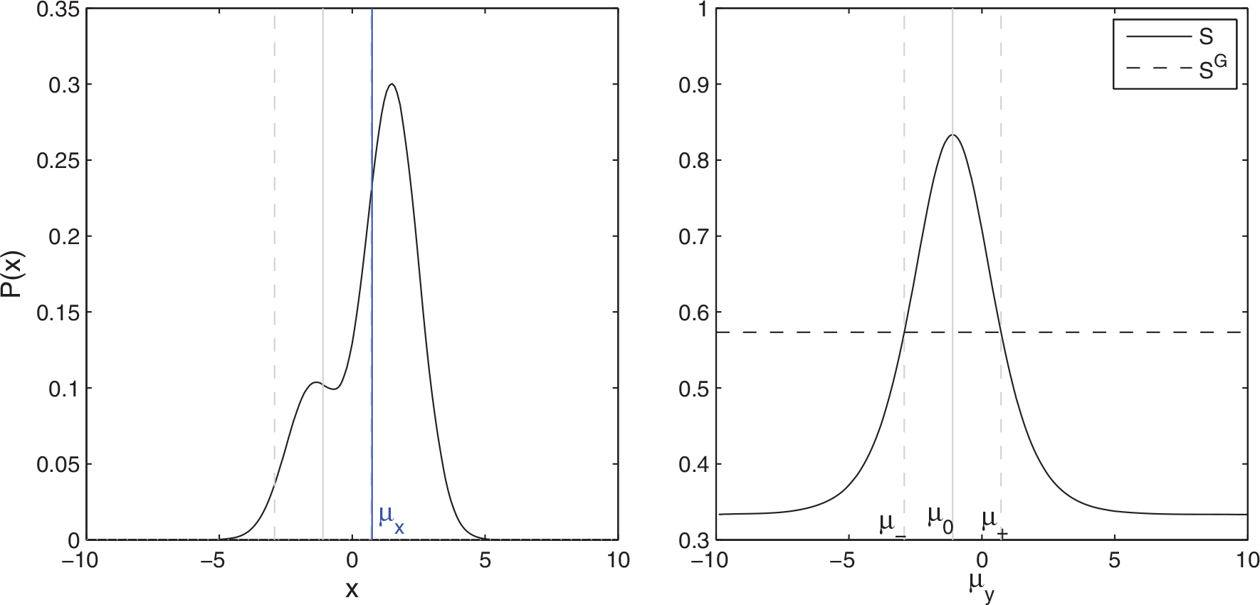
Fig. 2.
S (black), MI (red), RE (blue) all normalised by their Gaussian approximations. For the same parameters in Fig. 1. The black dashed line shows normalised by its Gaussian approximations.
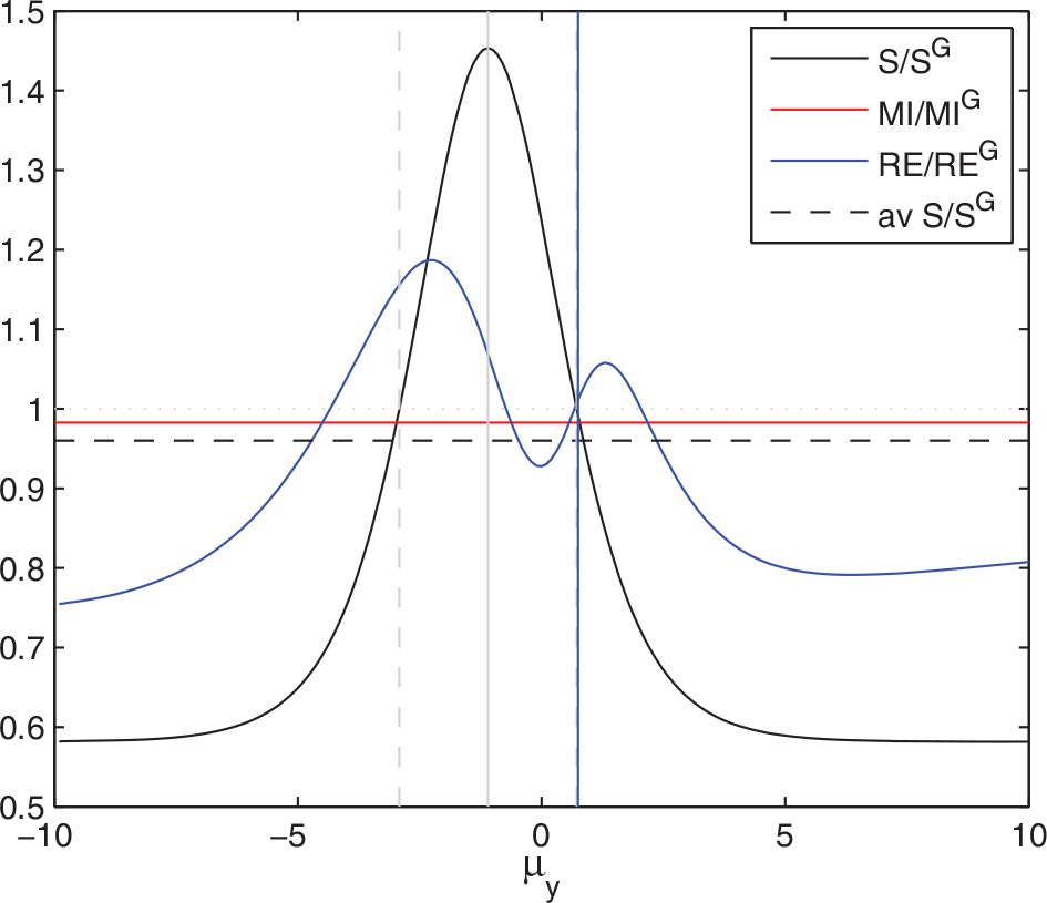
Fig. 3.
Contour plots of S (left) and RE (right) all normalised by their Gaussian approximations. These are given as a function of µ y and µ 2−µ 1 when (top row) and w when µ 2−µ 1=3 (bottom row). σ 2=1, k=2 as in Figs. 1 and 2. The grey lines mark µ y =µ x ±2σ x , where µ x and σ x are the mean and SD of the prior, respectively.
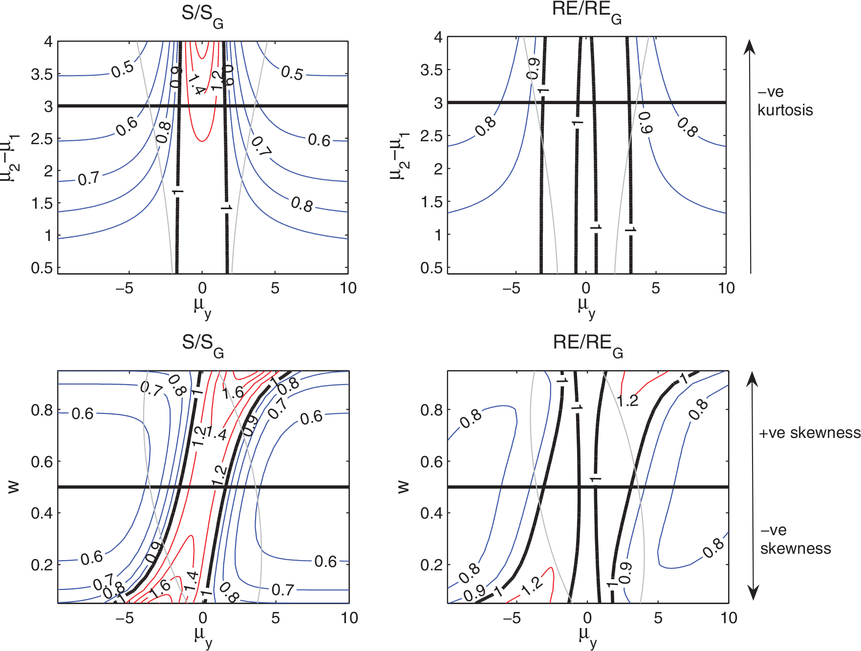
Fig. 4.
Contour plots of MI (left) and (right) all normalised by their Gaussian approximations. These are given as a function of µ 2−µ 1 (y-axis) and w (x-axis). σ 2=1, k=2. The grey lines mark the peak in the skewness (both positive and negative) of the prior.
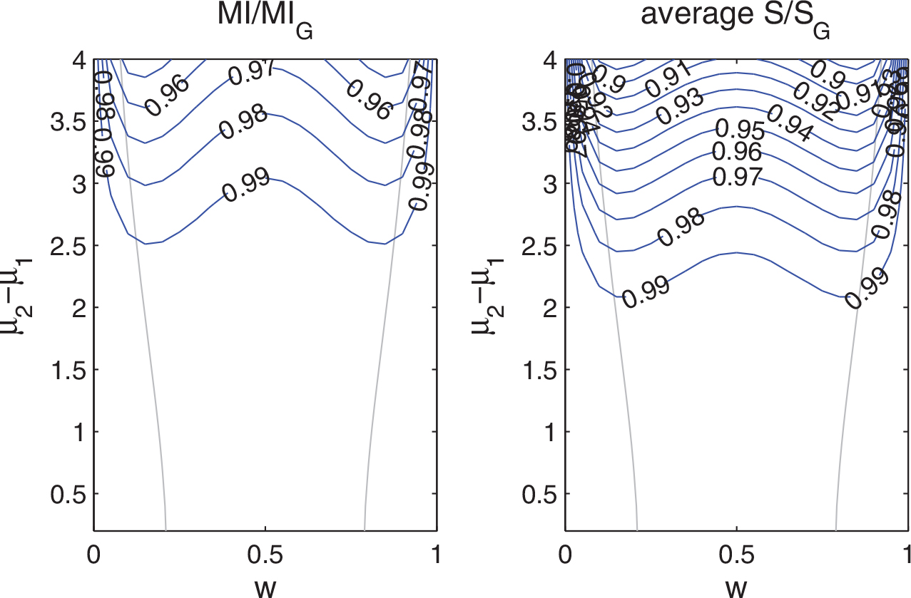
Fig. 5.
The evolution of the marginal prior distribution of χ 1: each panel gives a histogram representation of the particles at the time of the observations (bar plots). The blue stars give the value of the observations at each time. The black lines give a Gaussian approximation to the prior distribution and the red lines give a two-component Gaussian mixture fit to the prior distribution with identical variances, as described in Section 3.1.
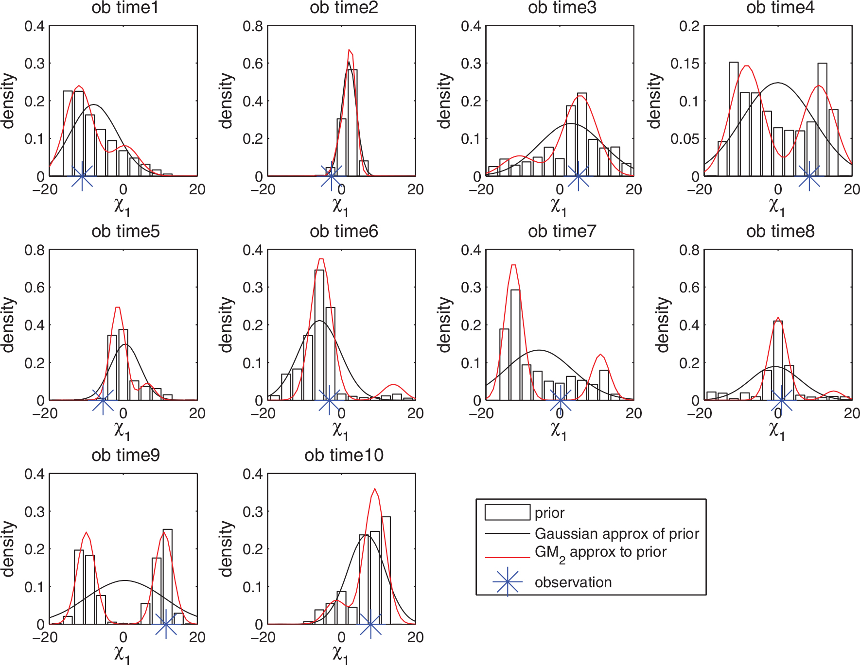
Fig. 6.
(a) The analysis (mean of particles) as a function of time (red), the true trajectory (grey) and observations of the truth (black crosses). (b) The prior variance as a function of observation time. (c) Approximations to the analysis sensitivity (black), relative entropy (blue) and mutual information (red dashed) assuming the prior distribution is Gaussian, with mean and covariance calculated from the weighted particles. (d) Approximations to the analysis sensitivity (black), relative entropy (blue) and mutual information (red dashed) calculated directly from the particle representation of the prior and posterior. Also plotted is the expected sensitivity (black dashed) and the ratio of the posterior variance to the observation error variance (grey dashed).
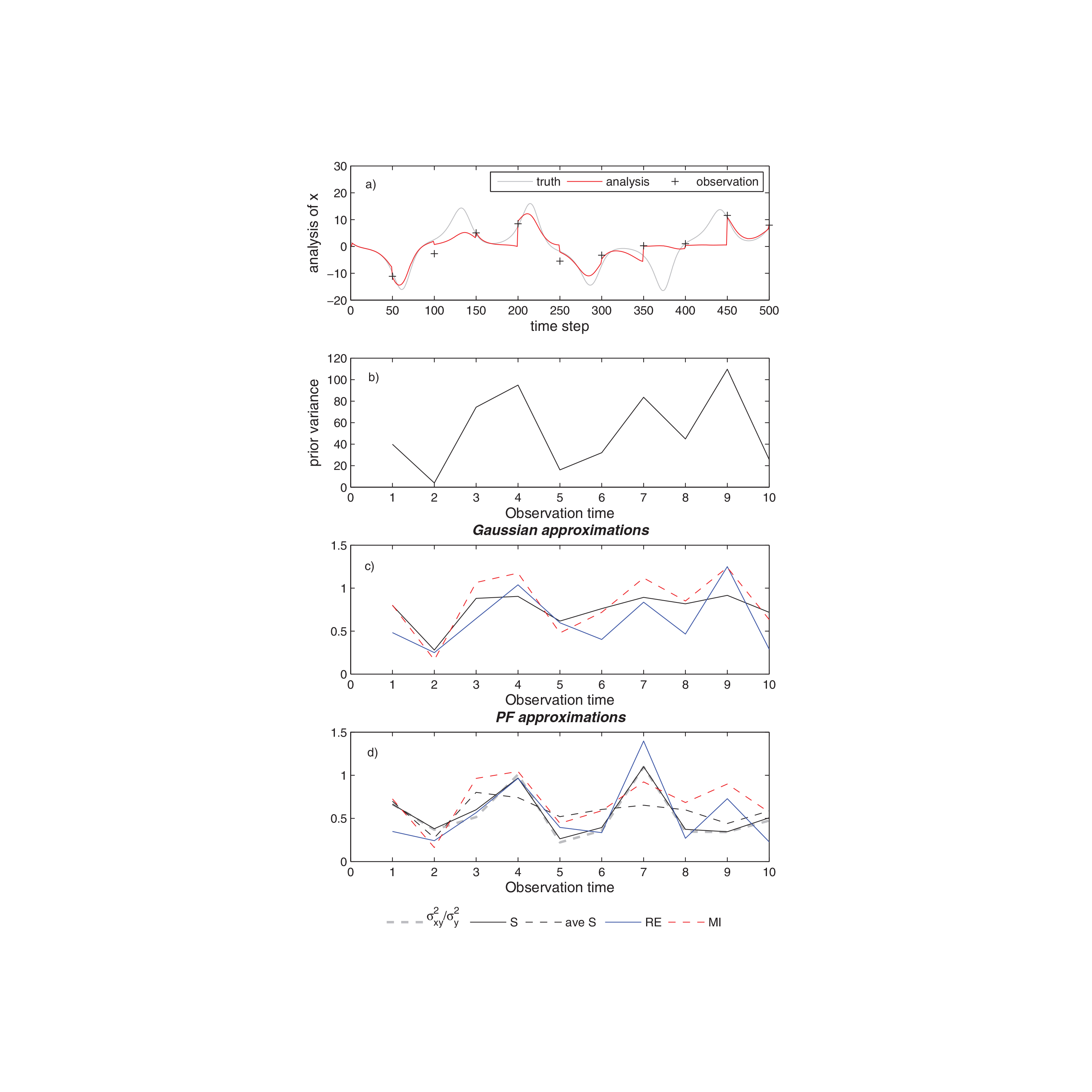
Fig. 7.
Top: the PF approximation to the observation impact divided by the Gaussian approximation for each measure. Line colours as in Fig. 6d. Bottom: the RMSE in the Gaussian approximation to the prior distribution as a function of observation time.
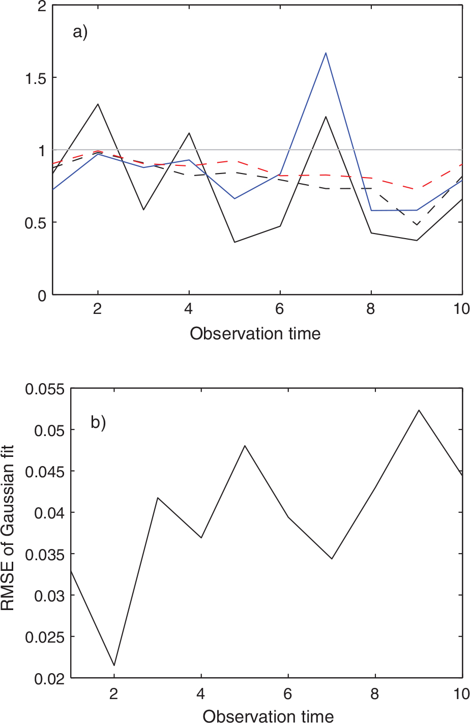
Fig. 8.
S (black), MI (red dashed), RE (blue) and (black dashed) as a function of the observation value all normalised by their Gaussian approximations. The black dashed-dot vertical line gives the realisation of the observation assimilated by the PF. Top: observation time 9. Bottom: observation time 7.