Table 1. Time mean RMSEs and spreads of the KF, and the minimum time mean RMSEs (over different β) of the KF-RN, in the AR1 model with different S a
[i] The KF and KF-RN have identical time mean spreads; therefore, only those of the KF are presented. In the bottom row, we also report the ranges of β in which the minimum time mean RMSEs of the KF-RN are achieved.
Fig. 1.
Time mean RMSEs of the KF and the KF-RN as functions of the noise level coefficient in the AR1 model, with different S a .
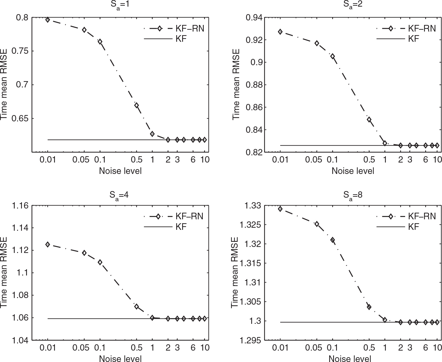
Fig. 2.
Left panels: Sample time series of the fraction coefficients of the KF-RN with β=0.1 (upper) and β=1 (lower), respectively. Right panels: The corresponding histograms of the fraction coefficient time series.
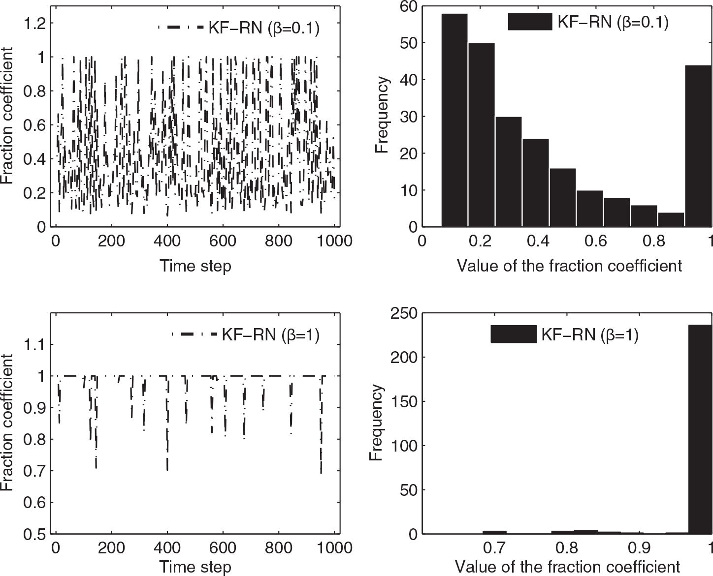
Fig. 3.
Time mean RMSEs of the normal EAKF and the EAKF-RN, as functions of inflation factor and half-width, in the full and 1/8 observation scenarios.
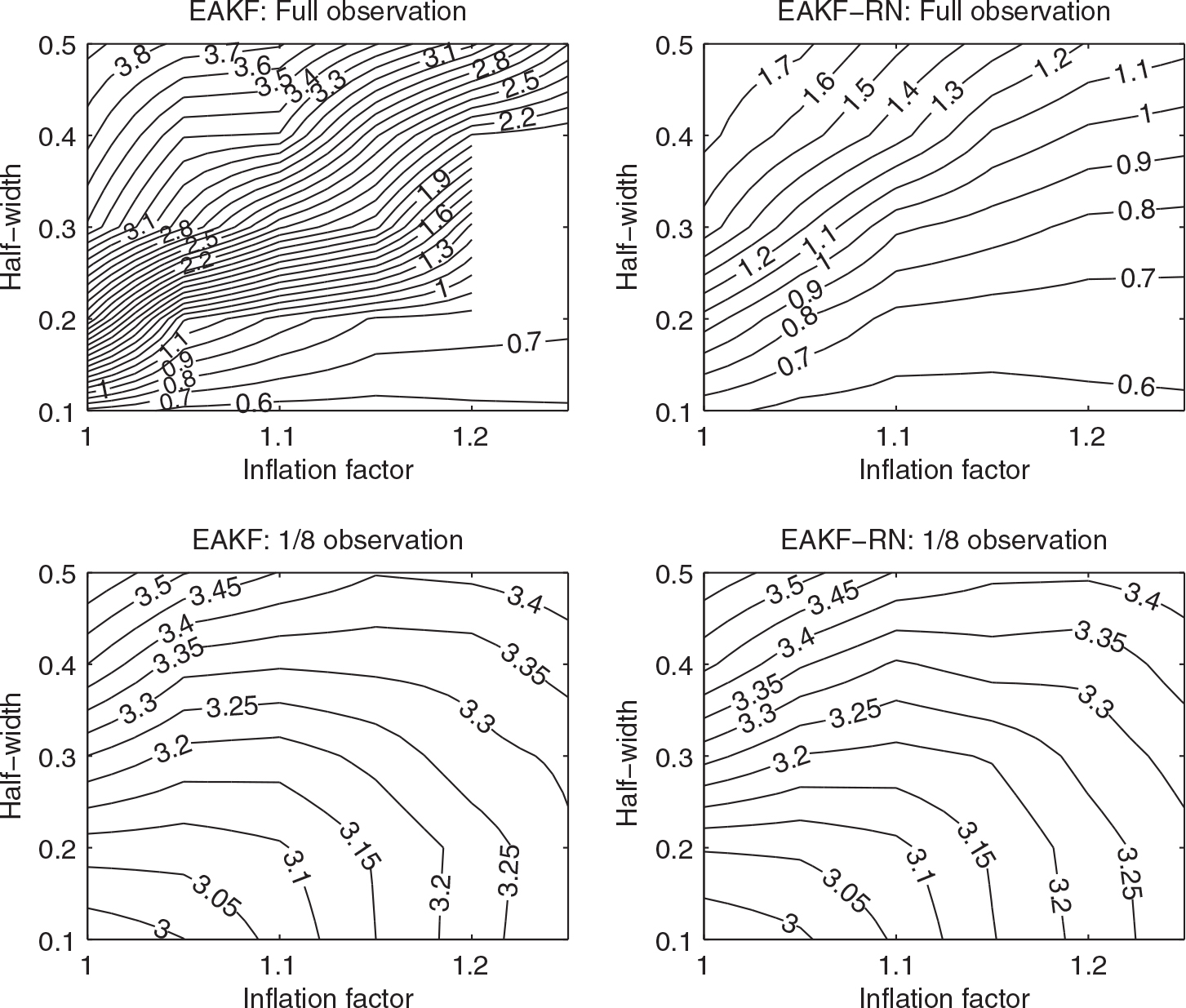
Table 2. Time mean RMSEs (spreads) of the normal EAKF and the EAKF-RN in the 1/2 observation scenario, as functions of the covariance inflation factor and the half-width of covariance localisation
Table 3. As in Table 2, except that it is in the 1/4 observation scenario
Fig. 4.
Time mean spreads of the normal EAKF and the EAKF-RN, as functions of inflation factor and half-width, in the full and 1/8 observation scenarios.
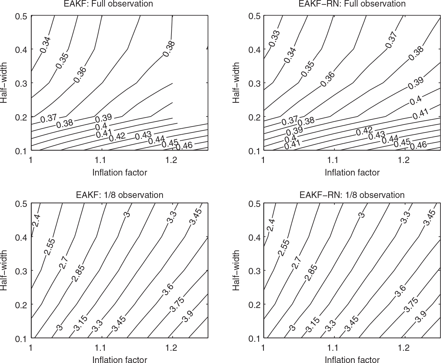
Fig. 5.
Time mean RMSEs of the normal EAKF and the EAKF-RN as functions of the noise level coefficient in different observation scenarios, with λ=1.15 and l c =0.1.
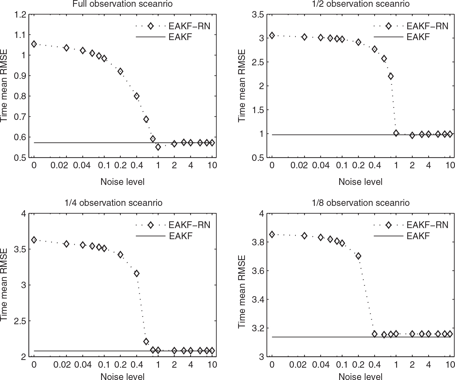
Fig. 6.
As in Fig. 5, but with λ=1.05 and l c =0.3 for both the filters. Note that in the 1/2 and 1/4 observation scenarios divergences of the normal EAKF are spotted; hence, no horizontal lines are indicated in the corresponding plots. The EAKF-RN also diverges in the 1/2 and 1/4 observation scenarios for β≥4.
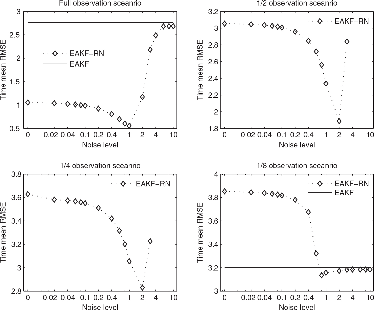
Fig. 7.
Upper left: sample time series of the RMSE of the normal EAKF in the 1/2 observation scenario; upper right: sample time series of the RMSE of the EAKF-RN (β=2) under the same experiment settings as the EAKF; lower left: corresponding fraction coefficient c k in the EAKF-RN (β=2); lower right: corresponding histogram of c k .
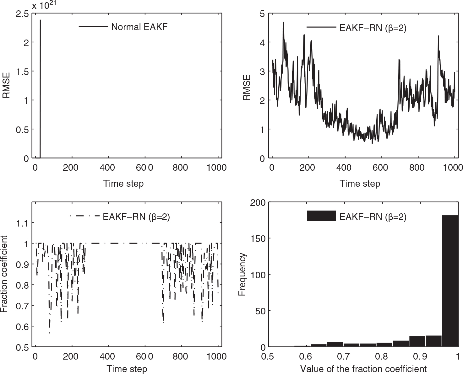
Fig. 8.
Upper: the RMSE of the EAKF (solid line with asterisks) and EAKF-RN (β=2, dotted line with plus signs) between the time instant k=1 and k=25; middle: difference in the RMSE (= RMSE of the EAKF – RMSE of the EAKF-RN) between k=1 and k=16; lower: the fraction coefficient of the EAKF-RN (β=2) between k=1 and k=25.
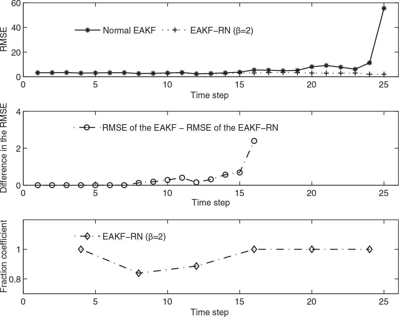
Fig. 9.
Time mean RMSEs of the EAKF and the EAKF-RN, as functions of the ensemble size in different observation scenarios.
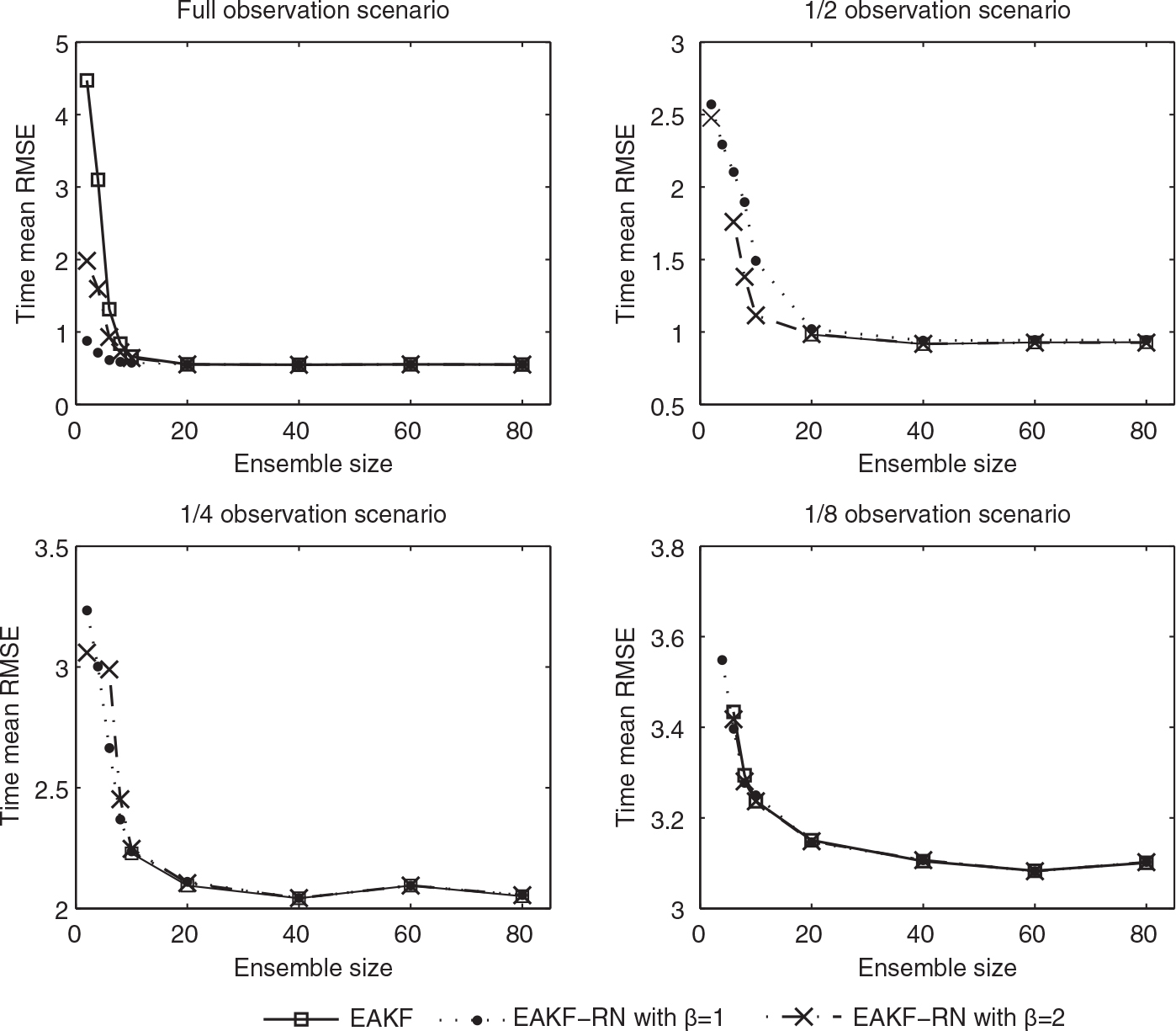
Fig. 10.
Time mean RMSEs of the normal EAKF, as functions of the assimilation step S a and the observation noise variance, in different observation scenarios.
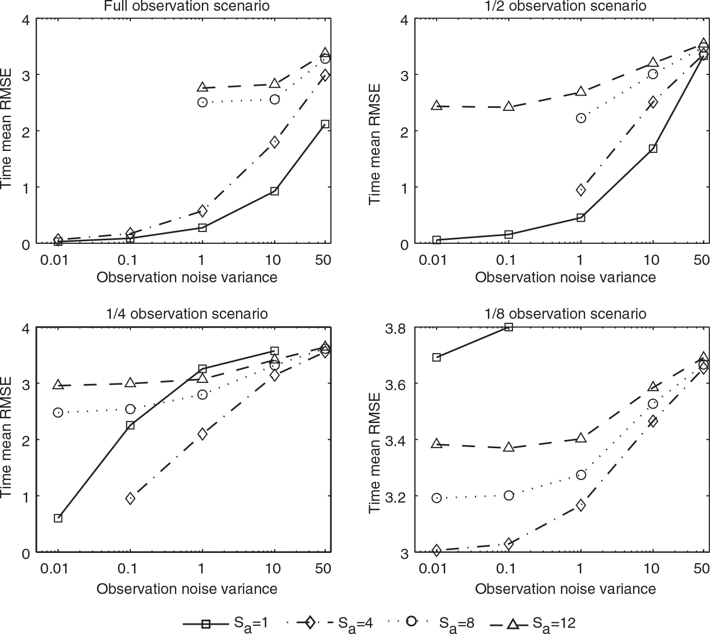
Fig. 11.
As in Fig. 10, but for the EAKF-RN with β=2.
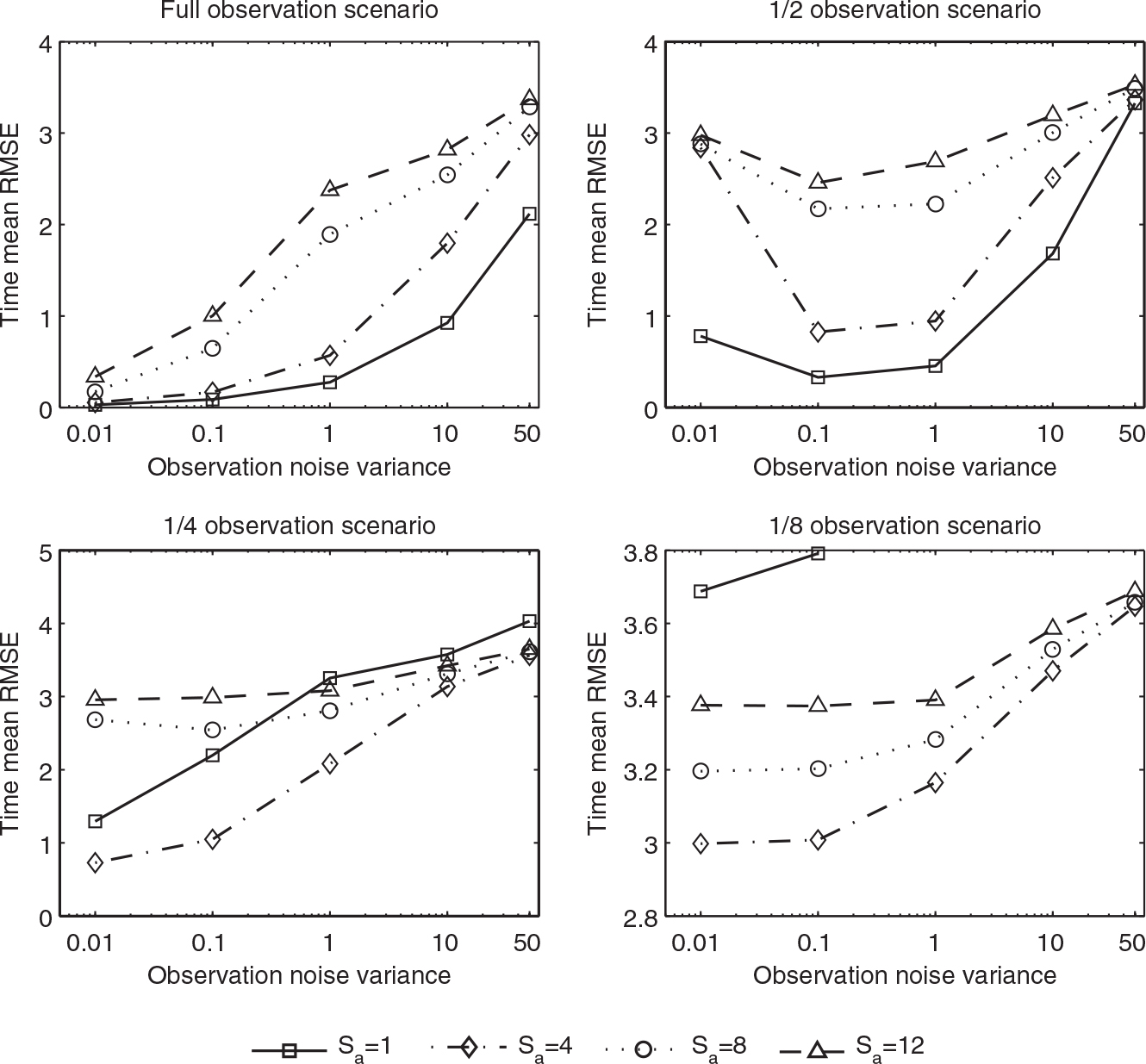
Fig. 12.
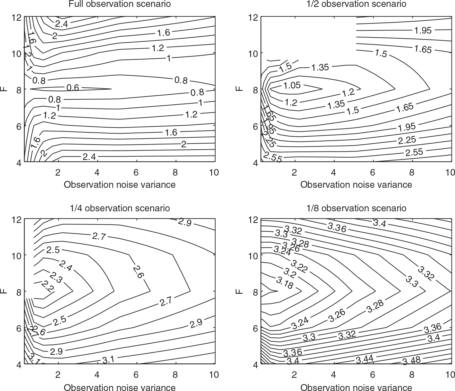
Time mean RMSEs of the EAKF, as functions of the (possibly) mis-specified driving force F and the observation noise variance γ, in different observation scenarios.
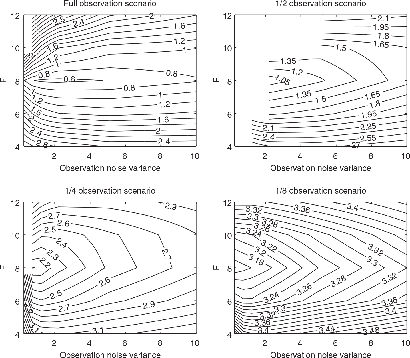
Fig. 13.
As in Fig. 12, but for the EAKF-RN with β=2.