Fig. 1.
Geographical coverage of the HIRLAM reference, called RCR, domain which is used in these experiments.
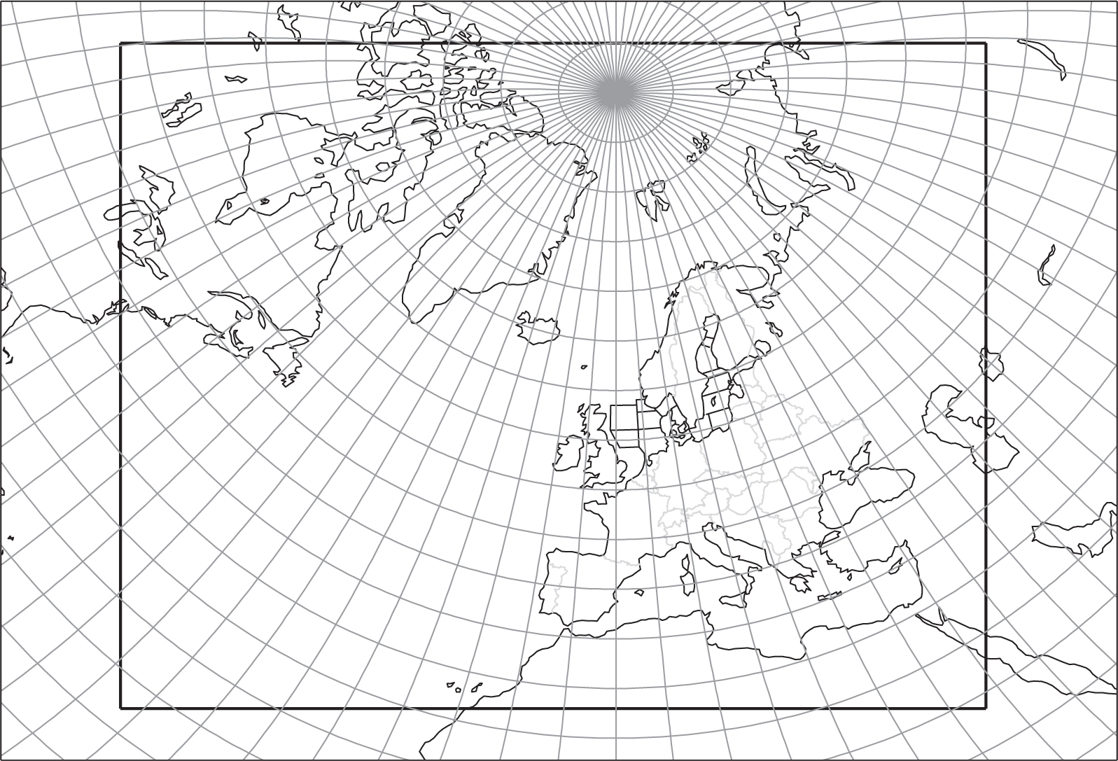
Fig. 2.
Integration area of the spectral HIRLAM tangent linear and adjoint model applied in 4D-Var, together with the horizontal resolution and the number of gridpoints for the setup used in the experiments presented in this work.
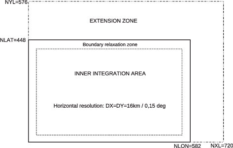
Fig. 3.
Left column: Horizontal variance power spectra, , for vorticity forecast differences at model levels 5 (≈90 hPa), 30 (≈630 hPa) and 50 (≈920 hPa), full line=ECMWF and dotted line=HIRLAM. Right column: cross-correlation of vorticity forecast differences between HIRLAM and ECMWF.
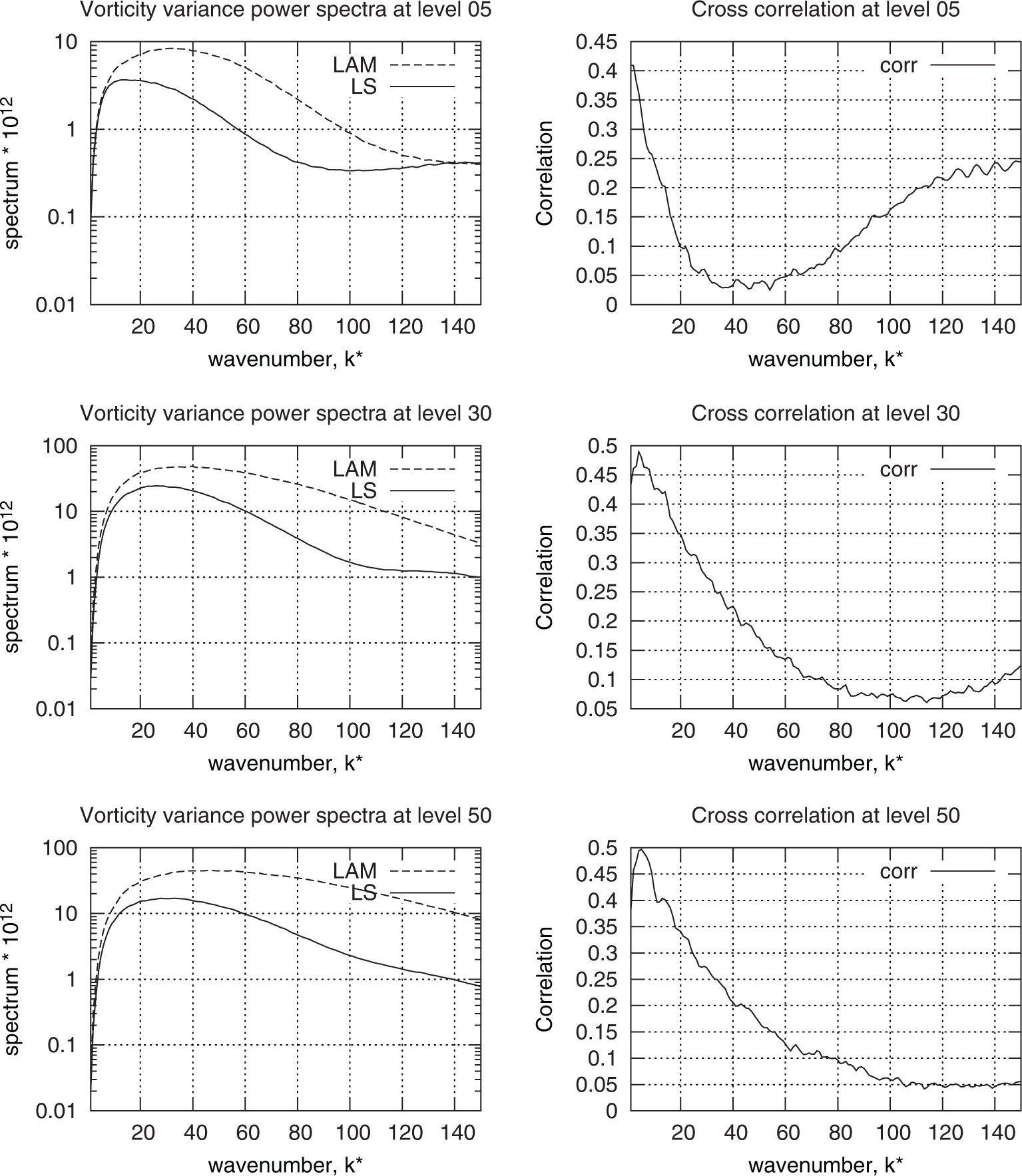
Fig. 4.
Vertical profiles of horizontally averaged standard deviation for vorticity forecast differences. These are both scaled in the minimisation to adjust the weight in the data-assimilation. Full line=ECMWF and dotted line=HIRLAM.
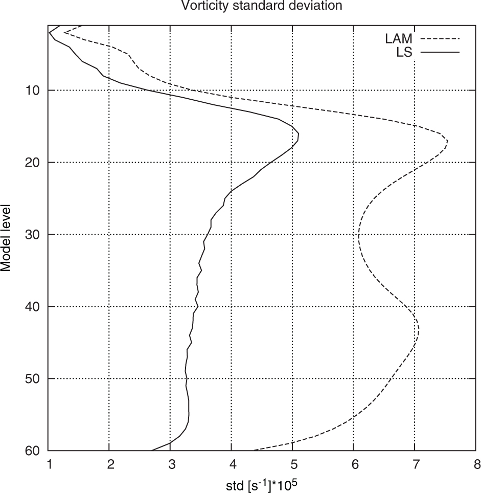
Fig. 5.
Horizontal spectral densities for vorticity forecast differences, γ. Full line=ECMWF, dotted line=HIRLAM. Before these are applied in the assimilation they undergo a scaling so that their sum, divided with the number of gridpoints, is equal to 1.
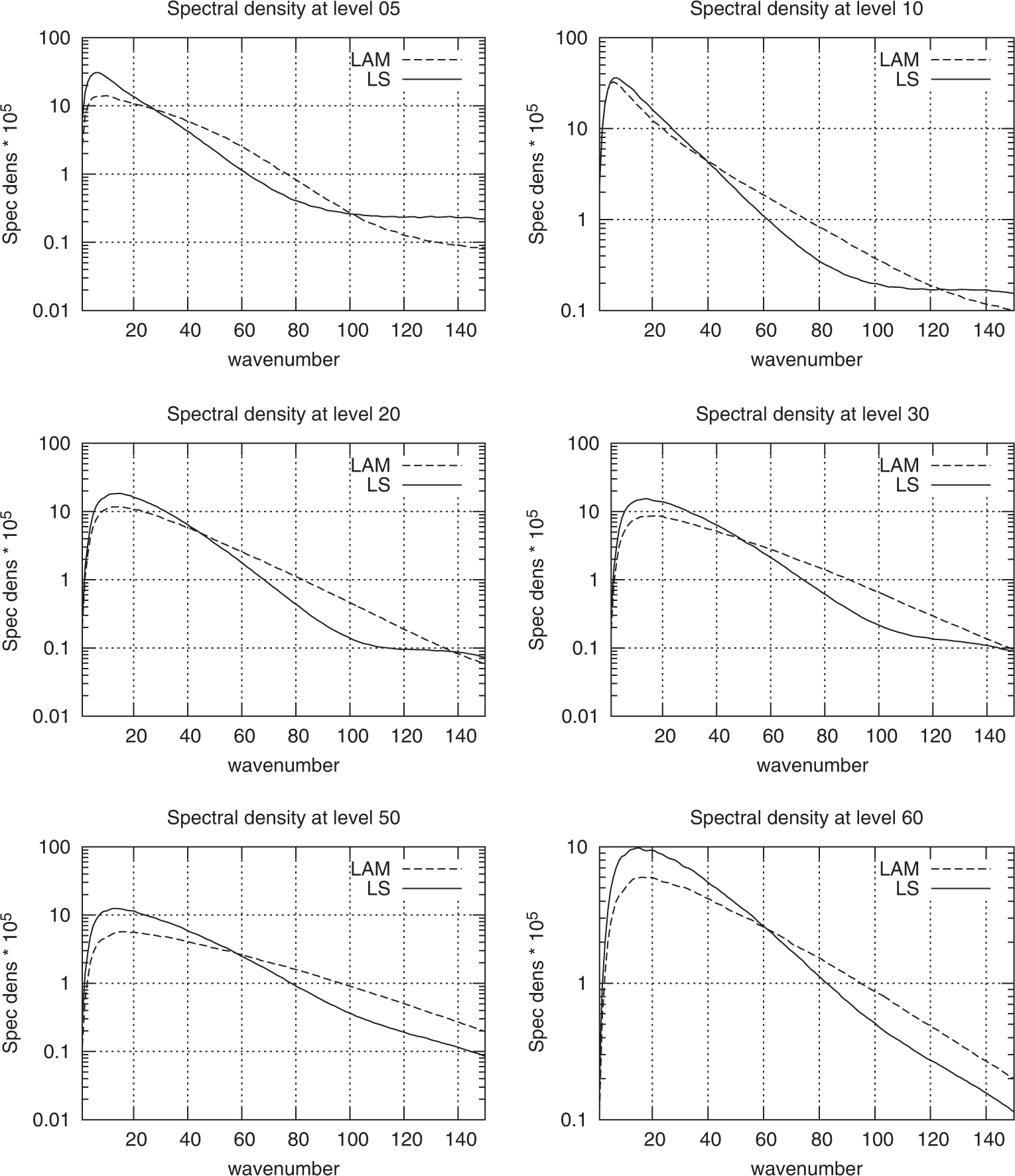
Fig. 6.
Eigenvalues for the vorticity forecast difference vertical covariance matrix, the first six leading modes. Mode number 1 is the leading mode and so on. The sum over the six modes are presented in the bottom figure.
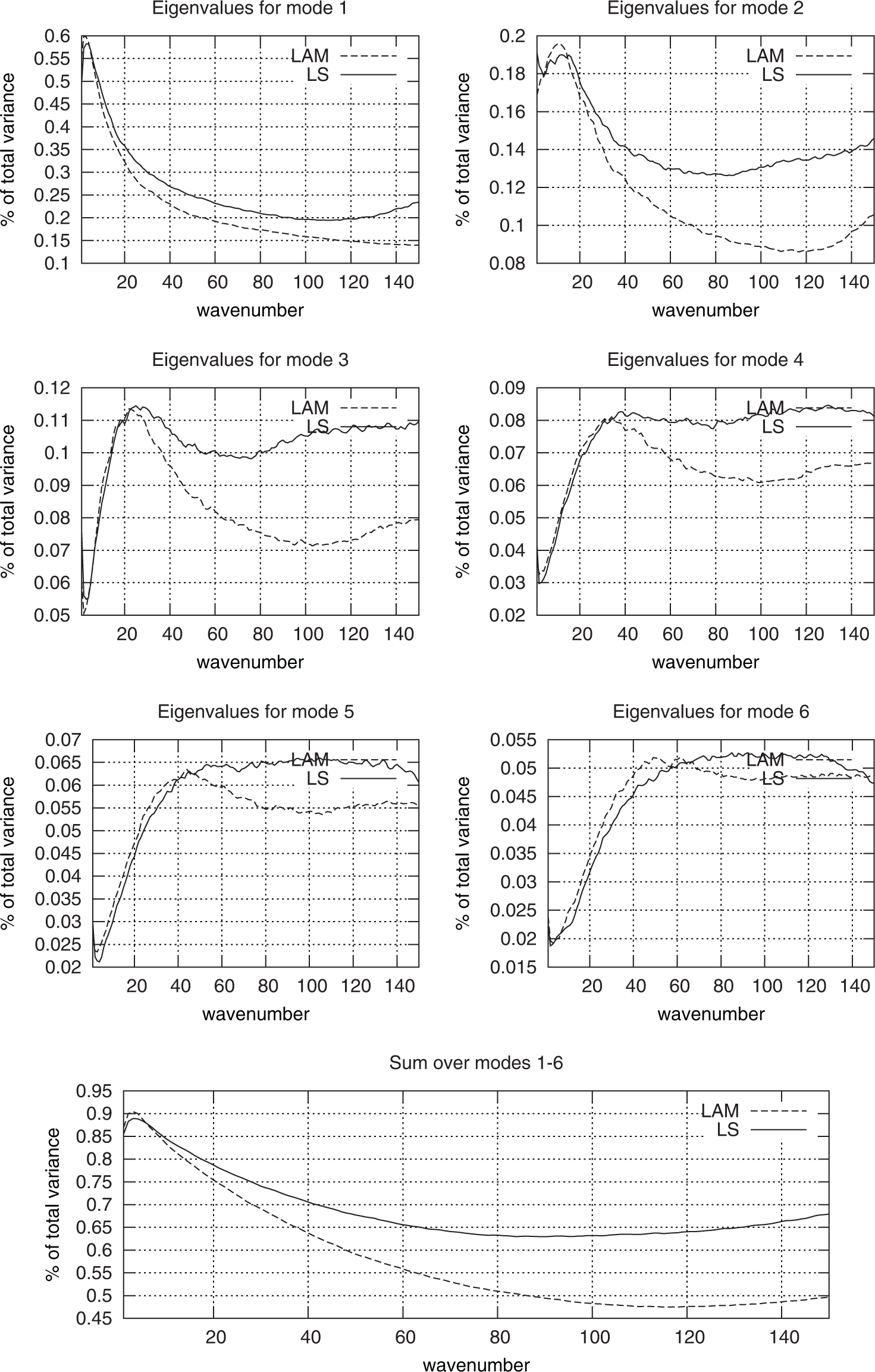
Fig. 7.
Eigenvectors for the first eight leading modes for the vorticity forecast difference vertical covariance matrix. The wave-number for each mode is the one that has the largest eigen-value, see Fig. 6.
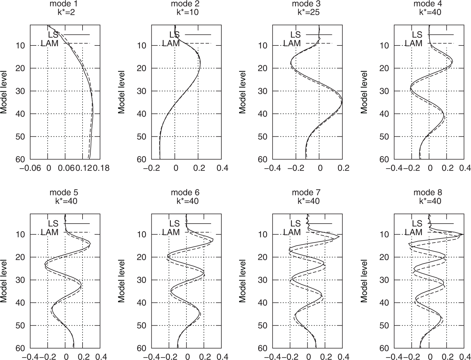
Fig. 8.
Analysis impact on upper air fields for a test case using 3D-Var and only the background and host model constraints, i.e. and thus no observations. Full line: RMS difference between x b and x ls . Dotted line: RMS difference between x a and x ls . x b is the background and first guess HIRLAM field and x ls is the ECMWF +06 h forecast used as constraint in J k . Notice that the inclusion of J k draws the analysed vorticity field closer to ECMWF.
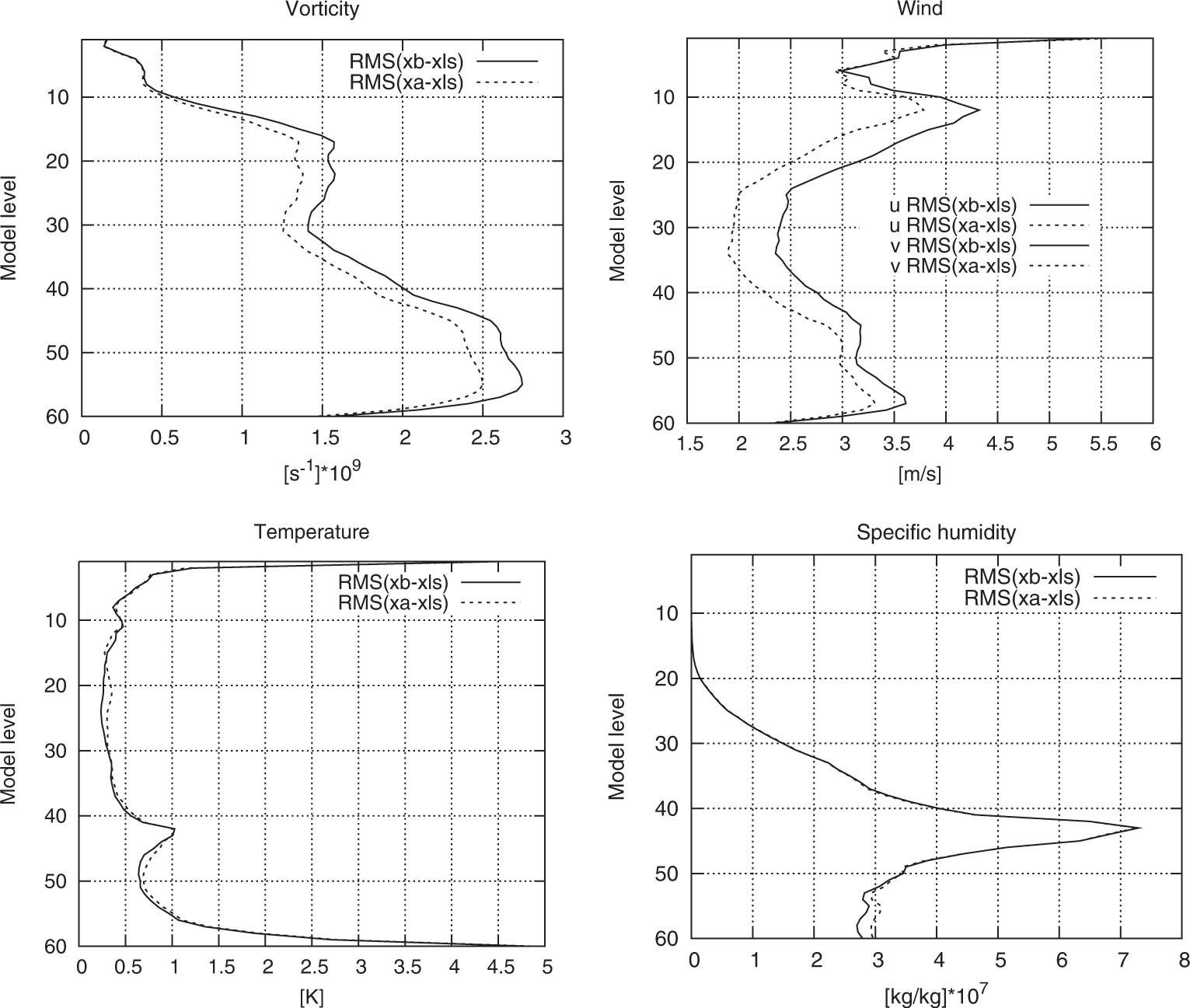
Fig. 9.
Spectrum of analysis impact on vorticity for a test case using 3D-Var and only the background and host model constraints, i.e. and thus no observations. Top figure, full line: absolute value of spectral coefficients for the difference . Top figure, dotted line: absolute value of spectral coefficients for the difference . Middle figure: absolute value of the analysis increments for vorticity, which corresponds to the difference between the full and dotted line in the top plot. Bottom figure: size of analysis increments relative to the first guess and host model vorticity fields, i.e. .
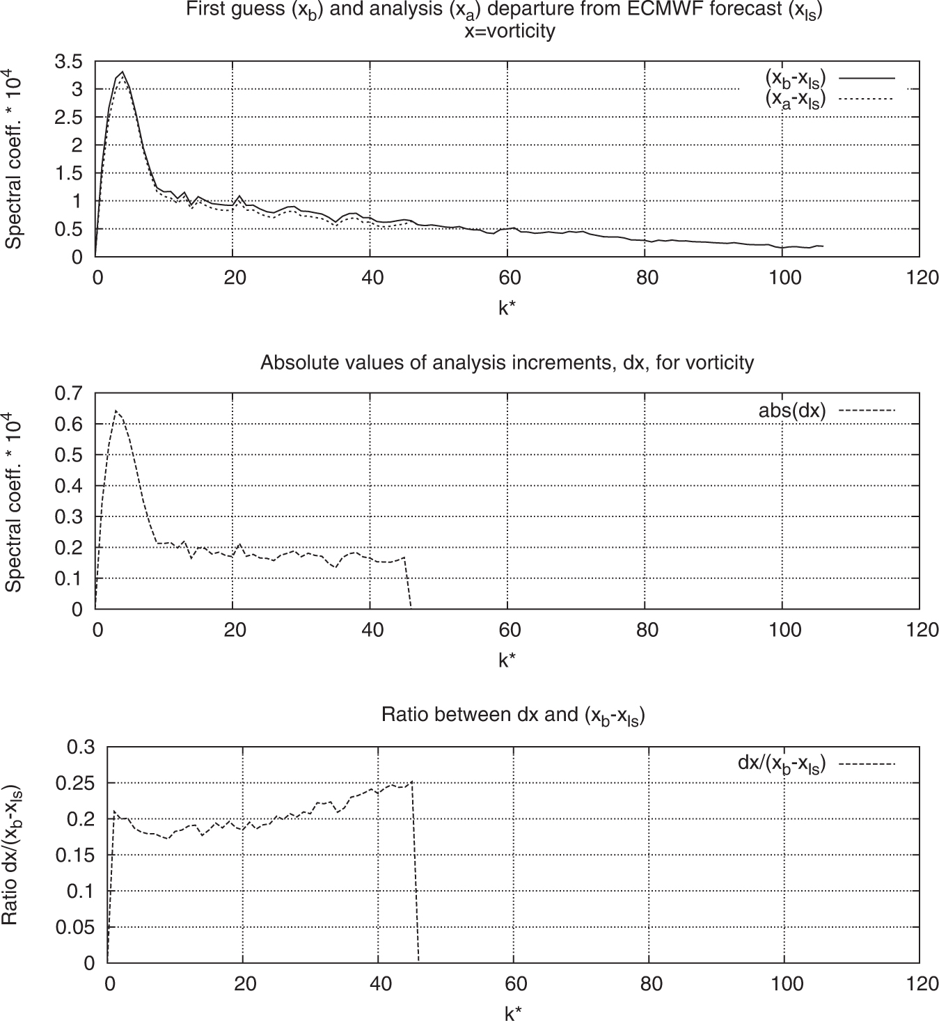
Fig. 10.
Cost-function behaviour for one case in the impact experiment. Here, a 4D-Var setting with two outer loops is used. As mentioned in Section 6.3, the resolution dependency of J b and J k is clearly shown here.
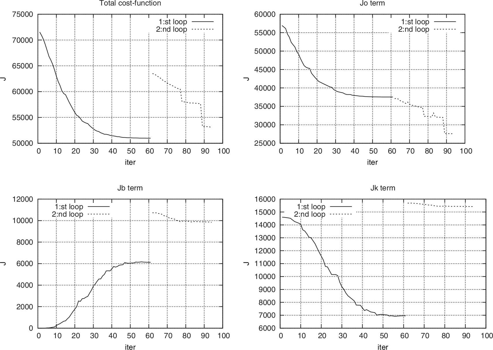
Fig. 11.
Verification of forecasts compared with observations of mean sea level pressure (MSLP). Upper lines are the Root Mean Square (RMS) error and the lower lines show the mean error, or bias. Full line: reference experiment (i.e. the host model constraint is not activated). Dotted line: same as reference except that J k is now actively used. The amount of observations used in the statistics is also shown using the right hand y-axis.
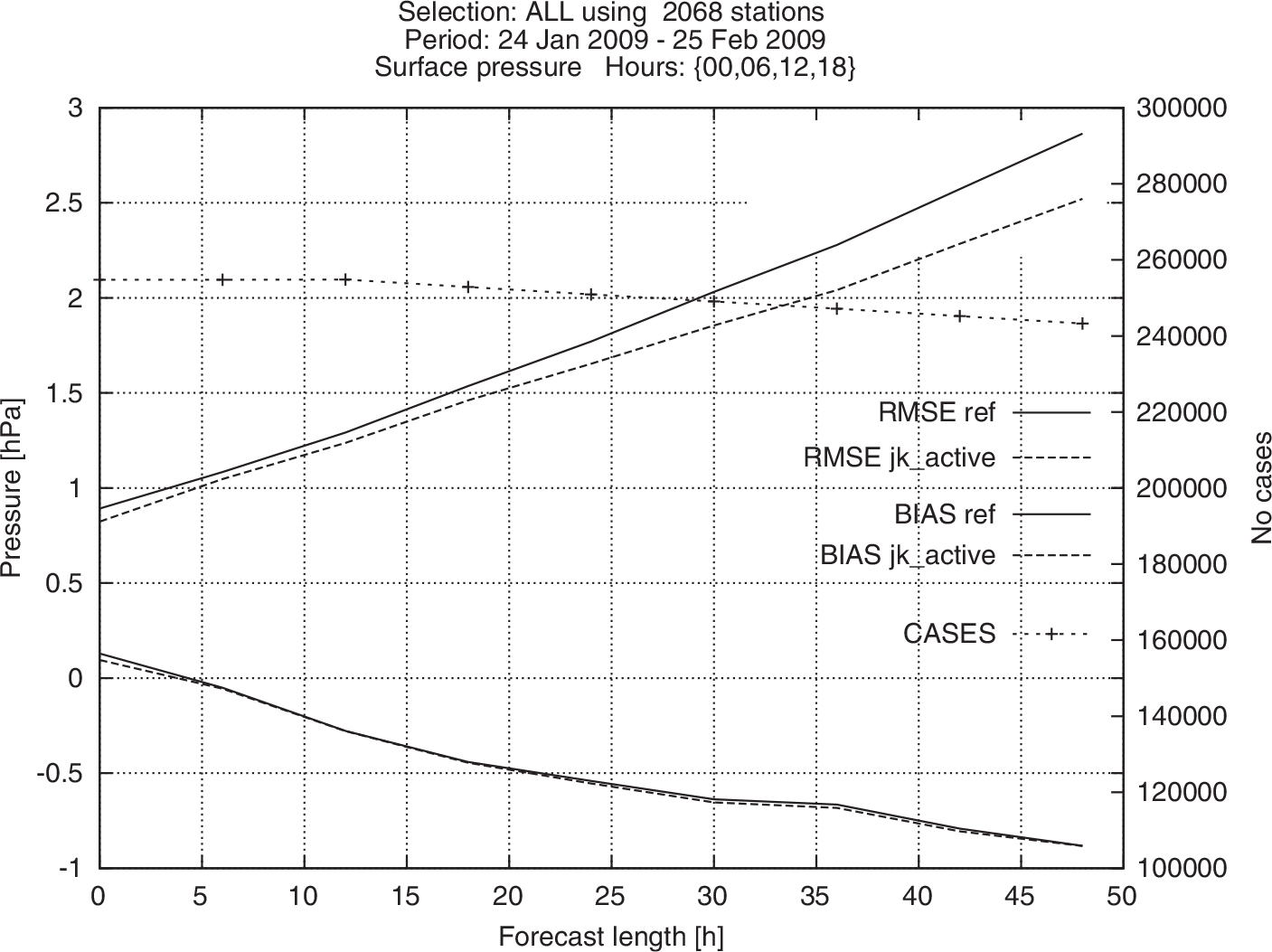
Fig. 12.
Verification of temperature forecasts compared with observations from radiosondes. To the right we have the Root Mean Square (RMS) error and to the left the mean error, or bias, averaged of all forecast lengths, valid at 00UTC (upper figure) and 12UTC (lower figure) are shown. Full line: reference experiment (i.e. the host model constraint is not activated.) Dotted line: same as reference except that J k is now actively used. The amount of observations used in the statistics is also shown using the upper x-axis.
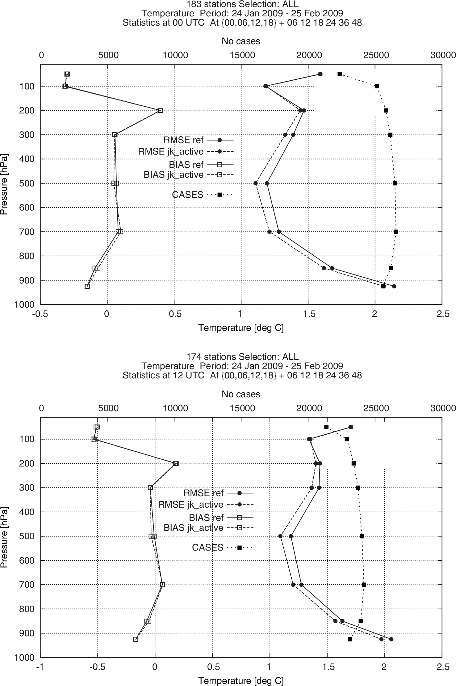
Fig. 13.
Time-series of surface pressure +24 h forecast errors compared with observations. The two lines at the top show the RMS errors, and the ones at the bottom the mean error. Full line: reference experiment (i.e. the host model constraint is not activated. Dotted line: same as reference except that J k is now actively used.
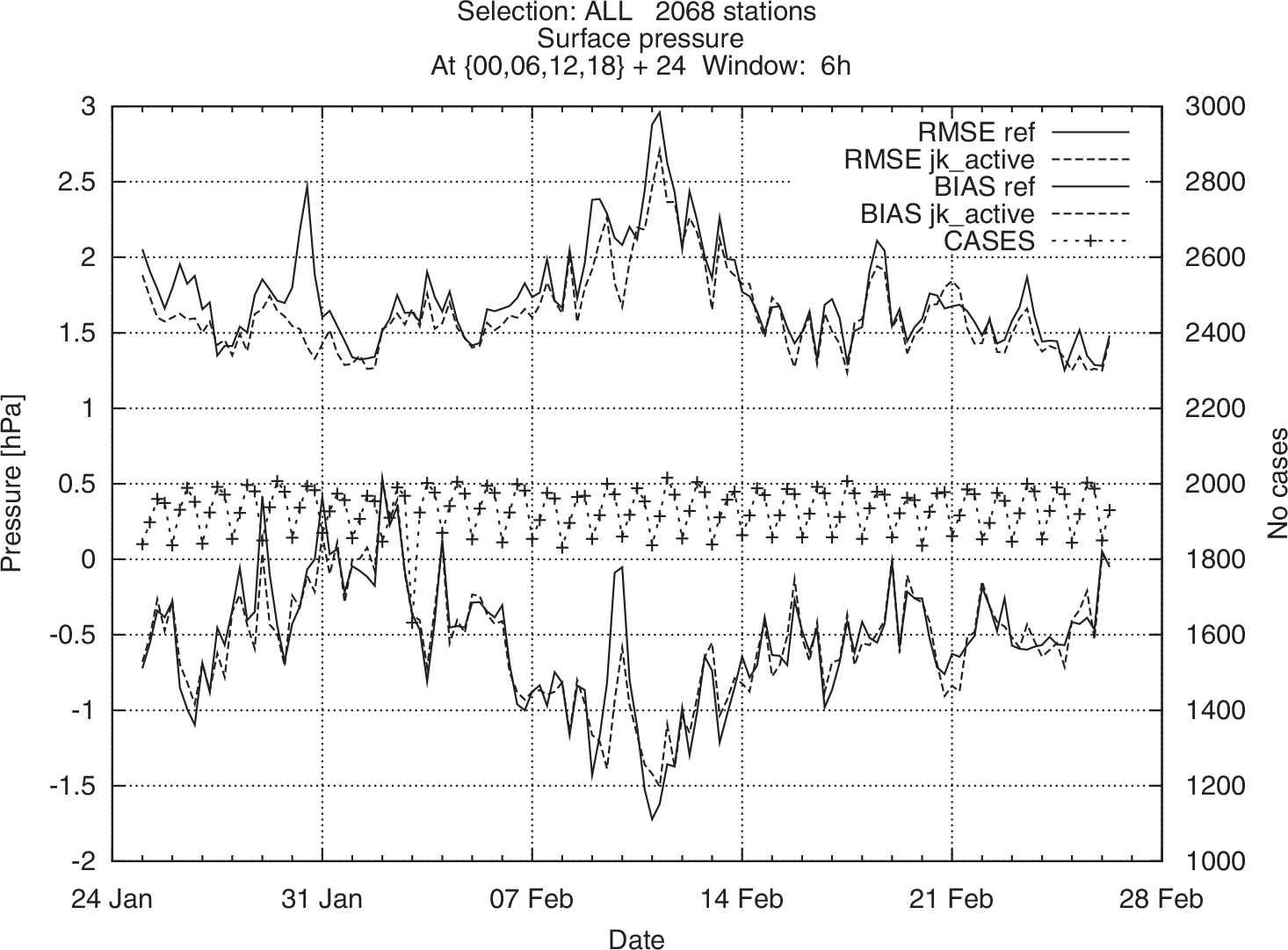
Fig. 14.
Analyzes of mean sea level pressure (MSLP) on 29 January 2009 12UTC. ref (top) refers to the run in which J k is not used, jk_active (middle) is the run that uses J k . The difference map (bottom) is the difference between jk_active and ref.
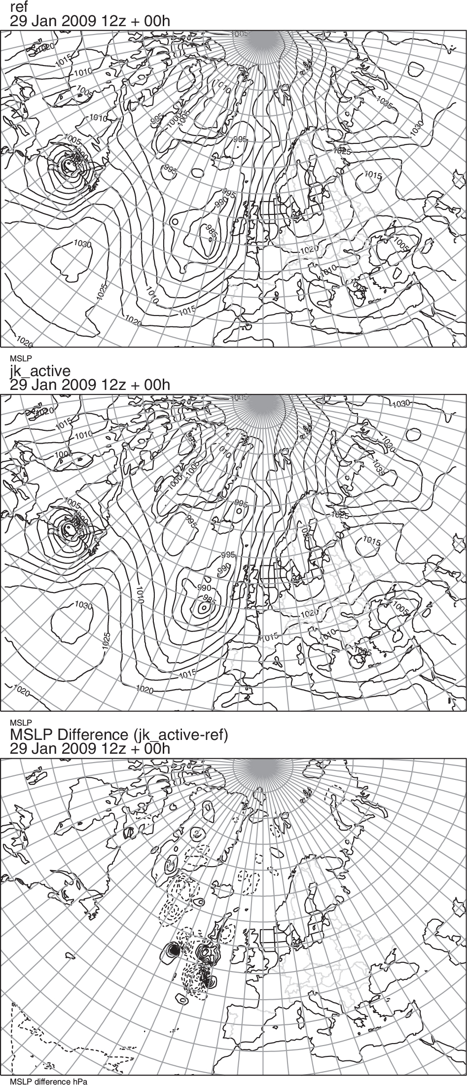
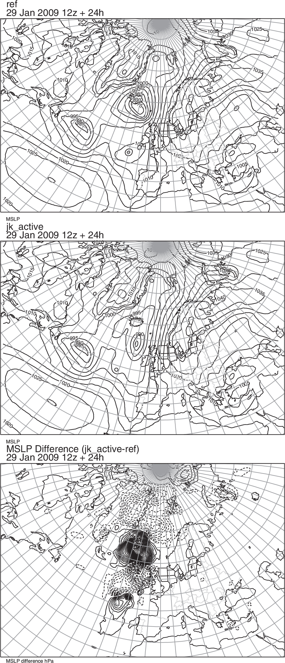
Fig. 15.
Mean sea level pressure fields for +24 h forecasts from 29 January 2009 12UTC, thus valid at 30 January 2009 12UTC.