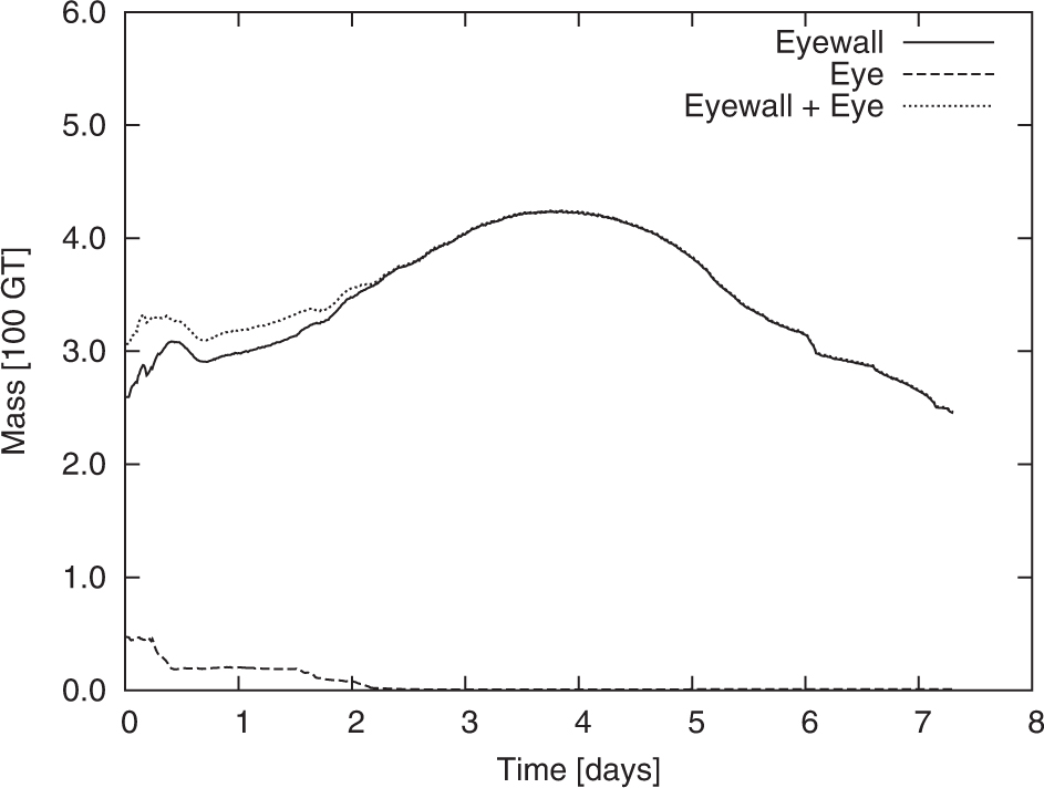
Fig. 1.
Sketch of the low-order tropical cyclone model, where s denotes specific entropy, R the potential radius and r the physical radius. The index letters b, i and a stand for boundary layer, inner and ambient region, respectively. Evaluation at saturation is indicated by an asterisk. Further notation is given in the text.
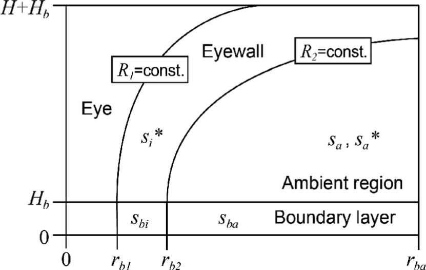
Table 1. Default model parameters
Fig. 2.
Maximum wind speed of the TC state as a function of for various timescales for shallow convective damping τ C . The solid line displays . The crosses and asterisks mark the analytical approximation given by eq. (46) for τ C =0.5 h and τ C =4 h, respectively.
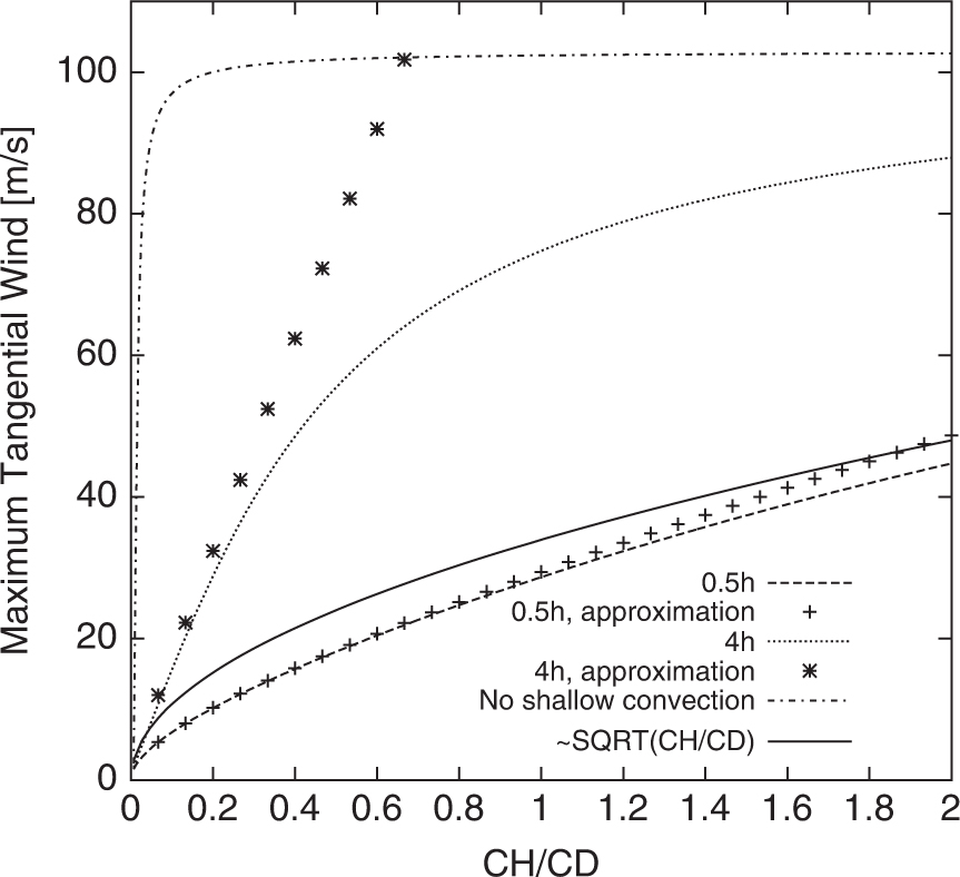
Fig. 3.
Equilibrium solutions for maximum tangential wind as a function of T s (°C) and h a (fraction by one) for (a) the non-neutral case I and (b) case N1 under the assumption of convective neutrality. Stable equilibria are coloured in dark grey and unstable equilibria in brighter grey.

Fig. 4.
Regime diagrams as a function of T s (°C) and h a (fraction by one) for (a) the non-neutral case I and (b) case N1 under the assumption of convective neutrality. The different regimes are labelled with different capital letters: The regime, where no stable low-pressure systems would form at all, is denoted as N-regime, in the A-regime we obtain two unstable equilibria, in the B-regimes (B1 and B2), the lower equilibrium is unstable and the upper is stable and in the C-regime, two unstable and two stable equilibria arise.
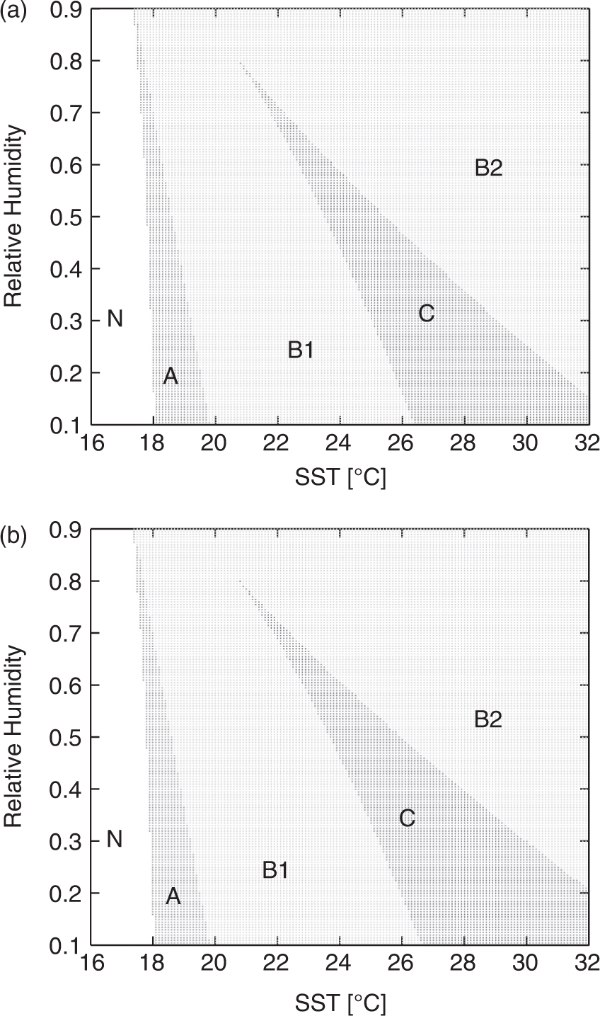
Fig. 5.
Bifurcation diagrams of maximum tangential wind speed (m s−1) as a function of T s (°C) for different β-values and a relative humidity in the ambient region of h a =45% for (a) the non-neutral case I and (b) case N1 under the assumption of convective neutrality. Stable equilibria are coloured in dark grey and unstable equilibria in brighter grey.
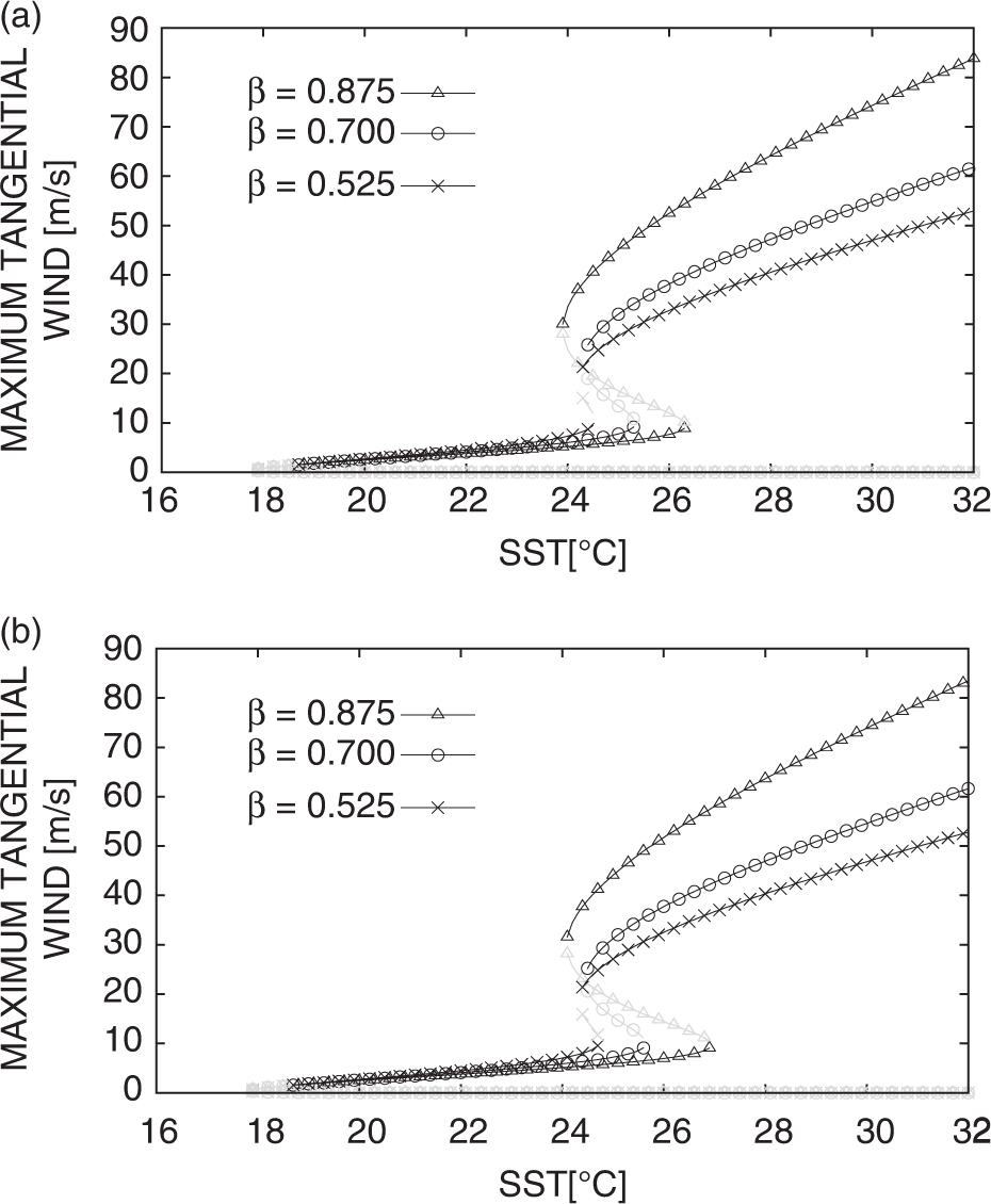
Fig. 6.
Bifurcation diagram of maximum tangential wind speed (m s−1) in case I as a function of T s (°C) for different τ C -values and a relative humidity in the ambient region of h a =45%. Stable equilibria are coloured in dark grey and unstable equilibria in brighter grey.
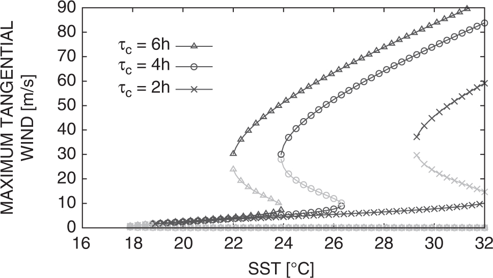
Fig. 7.
Regime diagrams in case I as a function of T s (°C) and h a (fraction by one) for different timescales in convective damping: (a) τ C =6 h, (b) τ C =4 h and (c) τ C =2 h. The different regimes are labelled as in Fig. 4.

Fig. 8.
Bifurcation diagram of maximum tangential wind speed (m s−1) in case I as a function of T s (°C) for different fix tropopause temperatures T t and a relative humidity in the ambient region of h a =45%. Stable equilibria are coloured in dark grey and unstable equilibria in brighter grey.
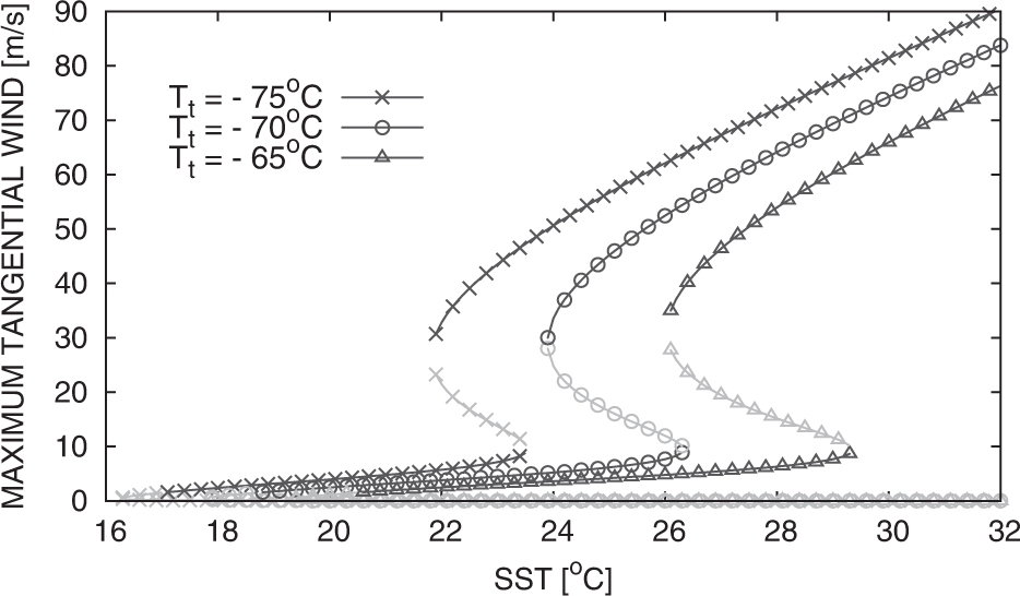
Fig. 9.
Regime diagrams in case I as a function of T s (°C) and h a (fraction by one) for different tropopause temperatures: (a) T t =−75°C, (b) T t =−70°C and (c) T t =−65°C. The different regimes are labelled as in Fig. 4.
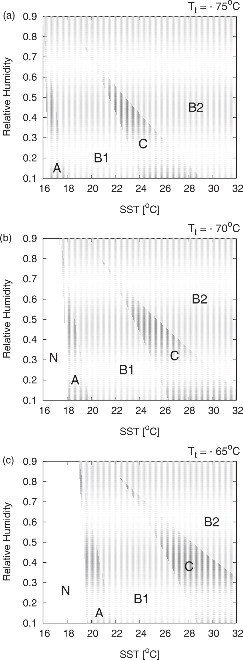
Fig. 10.
Equilibrium solutions for maximum tangential wind as a function of T s (°C) and h a (fraction by one) with τ C=8 h for (a) the neutral case N2 and (b) the hybrid case H. Stable equilibria are coloured in dark grey and unstable equilibria in brighter grey. Note that the SST-interval chosen in (a) to display case N2 extends into the unphysical range of temperatures below the freezing point.
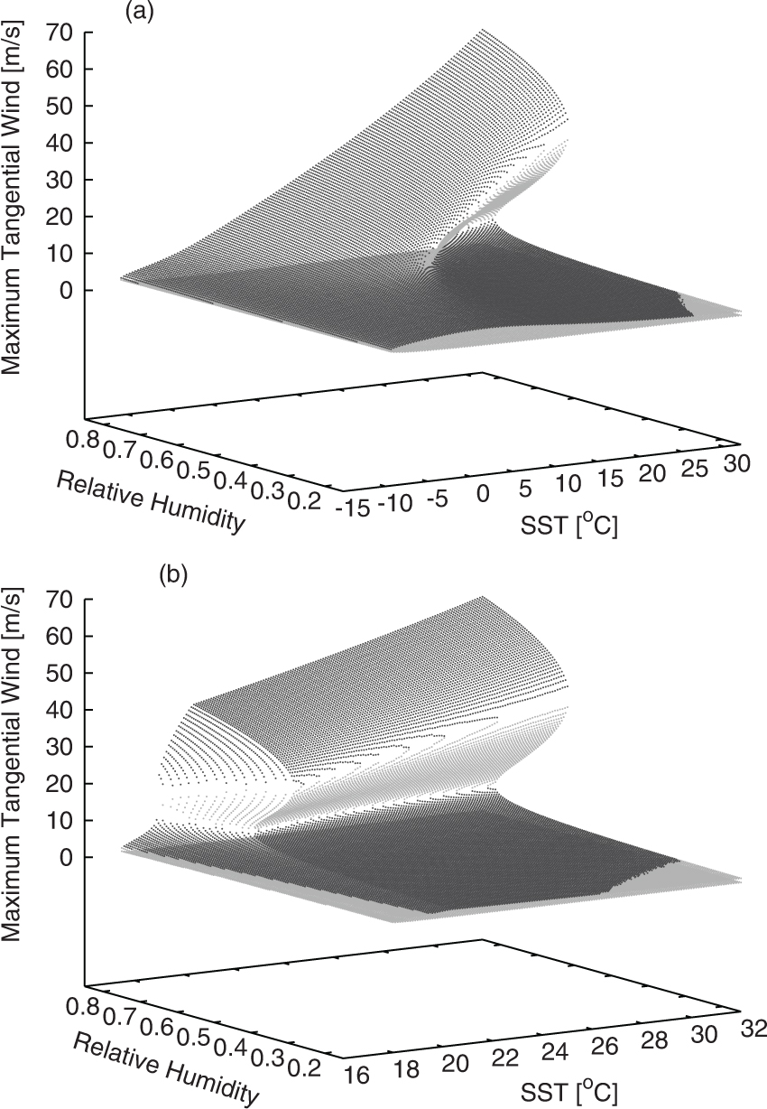
Fig. 11.
Regime diagrams as a function of T s (°C) and h a (fraction by one) with τ C=8 h for (a) the neutral case N2 and (b) the hybrid case H. The different regimes are labelled as in Fig. 4.
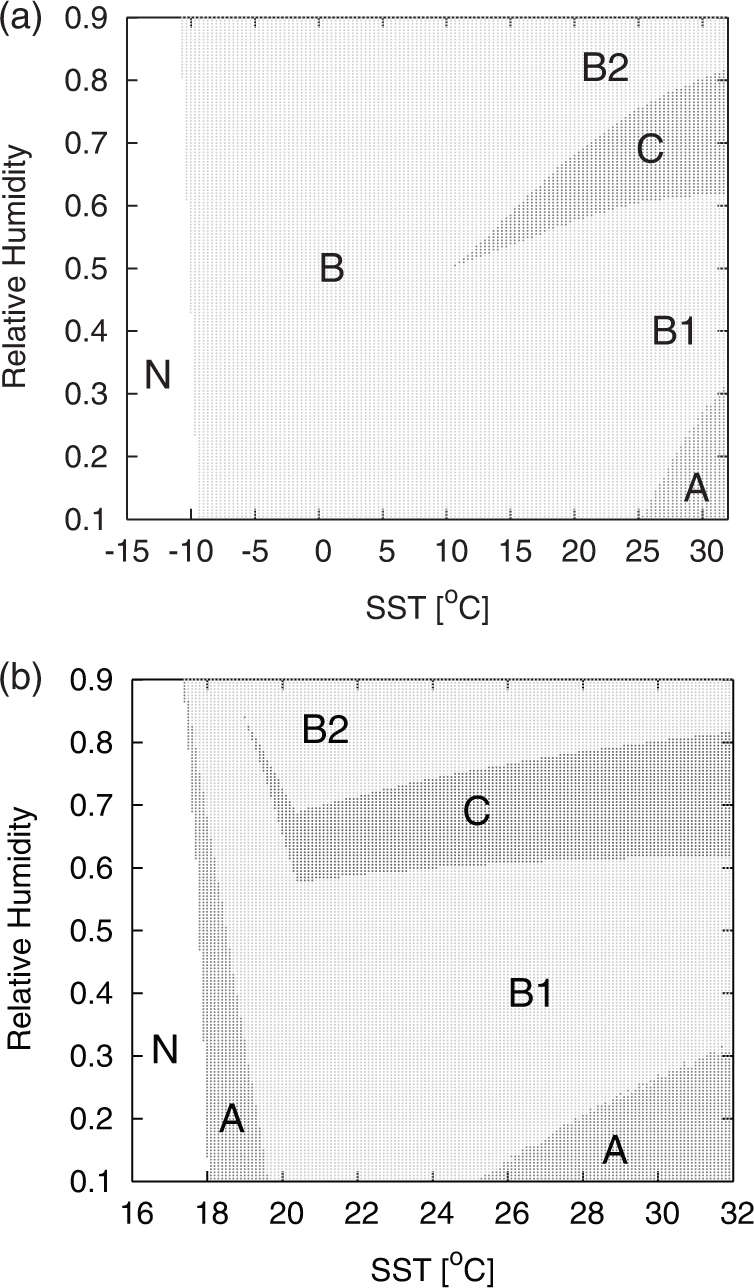
Fig. 12.
Regime diagrams in case H as a function of T s (°C) and h a (fraction by one) for different timescales in convective damping: (a) τ C =10 h, (b) τ C =8 h and (c) τ C =6 h. The different regimes are labelled as in Fig. 4.
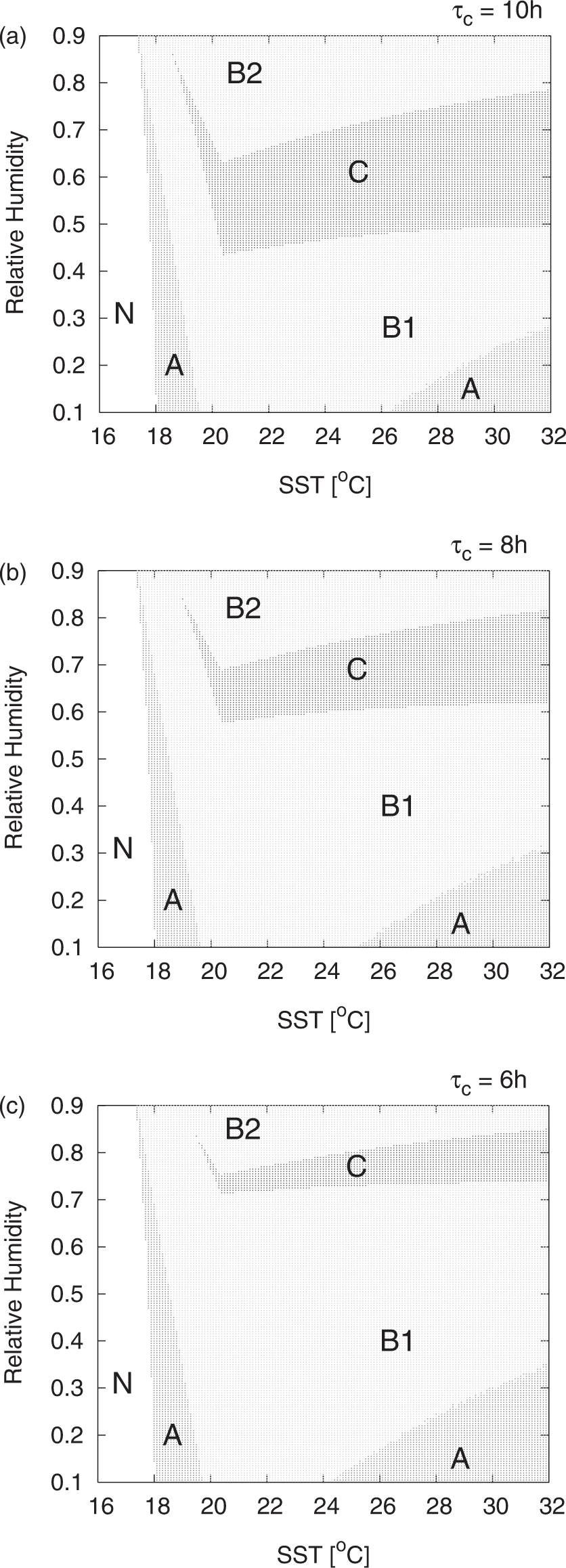
Fig. 13.
Time evolution of entropy for various transfer coefficients C H and C D . The curves display time integrations of the dynamical system (50)–(52), which is valid at small amplitudes.
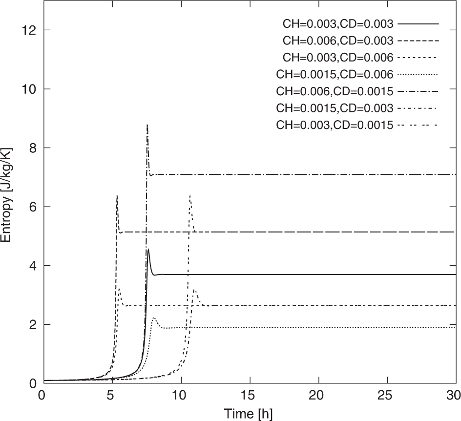
Fig. 14.
Time development (in days) of v b2 (in m s−1) in case I with h a =45% started near an unstable equilibrium for (a) T s=25°C and (b) T s=28°C. Equilibrium solutions in the upper panel (a) are located in the C-regime (see Figs 3a and 4a), and model runs initialised by small perturbations with respect to the upper repellor are plotted with dashed lines and those started near the lower equilibrium are plotted with solid lines. In the lower panel (b), equilibrium solutions exist in the B2-regime with only one repellor. For each repellor, runs were initialised by one negative perturbation and six gradually increased positive perturbations.
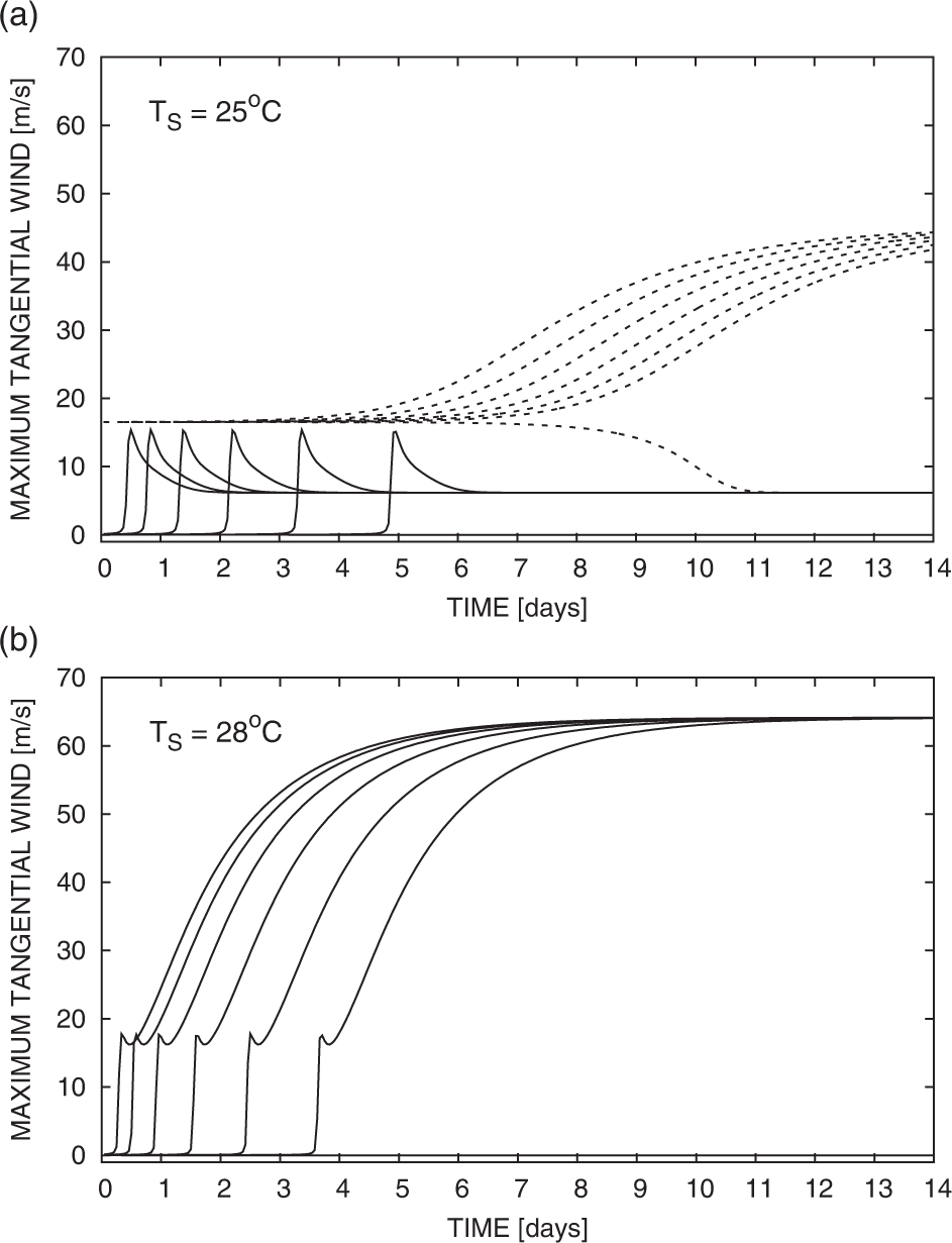
Fig. 15.
Vertical velocity at z=1250 m (black isolines, contour interval 1 m s−1) and saturation entropy (shadings, J kg−1 K−1) at z=5250 m as a function of potential radius and time for the HURMOD experiment.
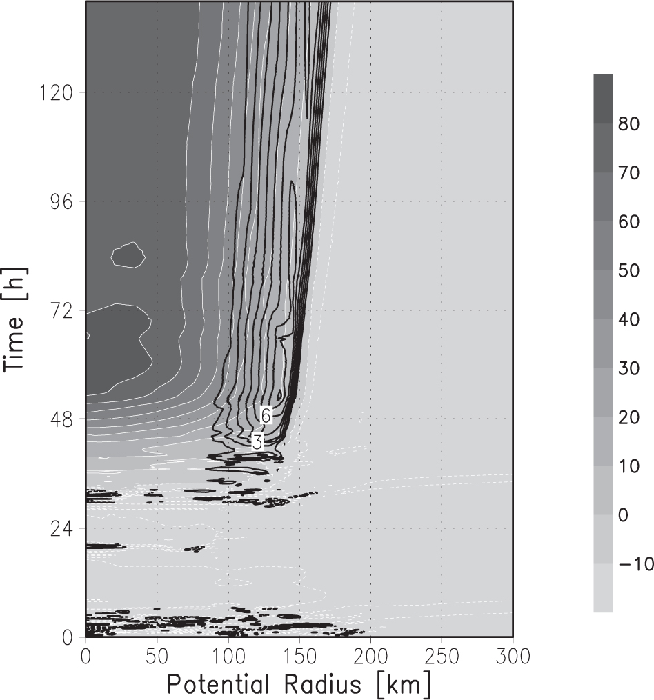
Fig. 16.
Mass stream function (black isolines, contour interval 0.25×10⁹ kg s−1) and specific entropy (shadings, J kg−1 K−1) time averaged over the period 75–140 h as a function of potential radius and height for the HURMOD experiment.
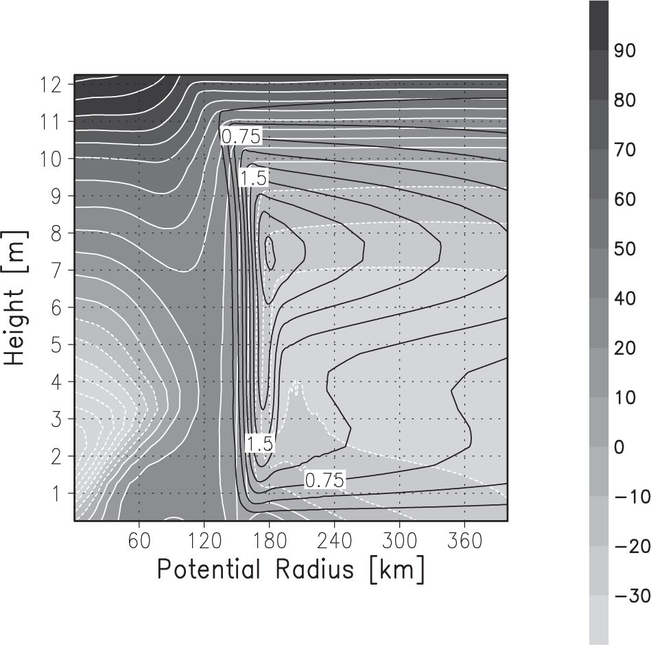
Fig. 17.
Radial profiles of tangential wind at z=1250 m for t=38 h, t=44 h and t=50 h of the HURMOD experiment (solid lines). The dashed lines and dotted lines display the estimate for and , respectively.
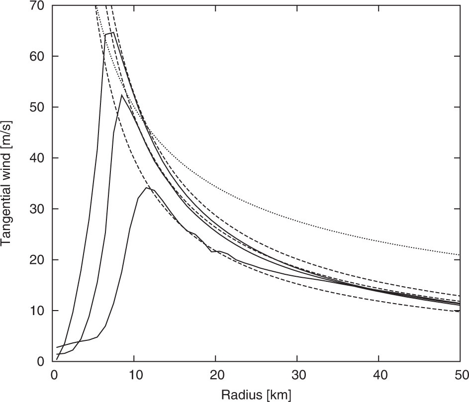
Fig. 18.
Mass (in 100 gigatons) of the eyewall (solid line), eye (dashed line) and the sum of both (dotted line) as a function of time for the HURMOD experiment.