
Fig. 1.
HIgh Resolution Limited Area Model mean sea level pressure (MSLP) forecast on 3 December 1999, 00 UTC + 11 h. The contour interval is 5 hPa.
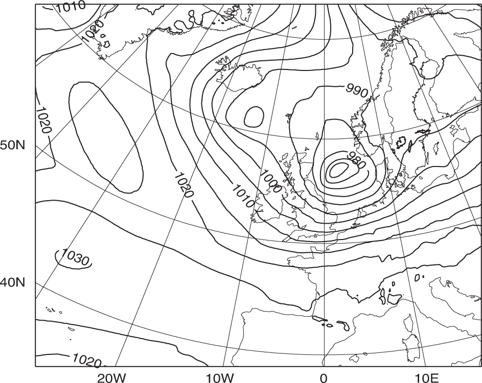
Fig. 2.
3D-Var surface pressure assimilation increments for 3 December 1999, 11 UTC from a single surface pressure observation increment of −5 hPa at 57°N 3°E for 3 December 1999, 11 UTC. The assumed standard deviation of the observation error is 0.5 hPa. The contour interval is 1 hPa.
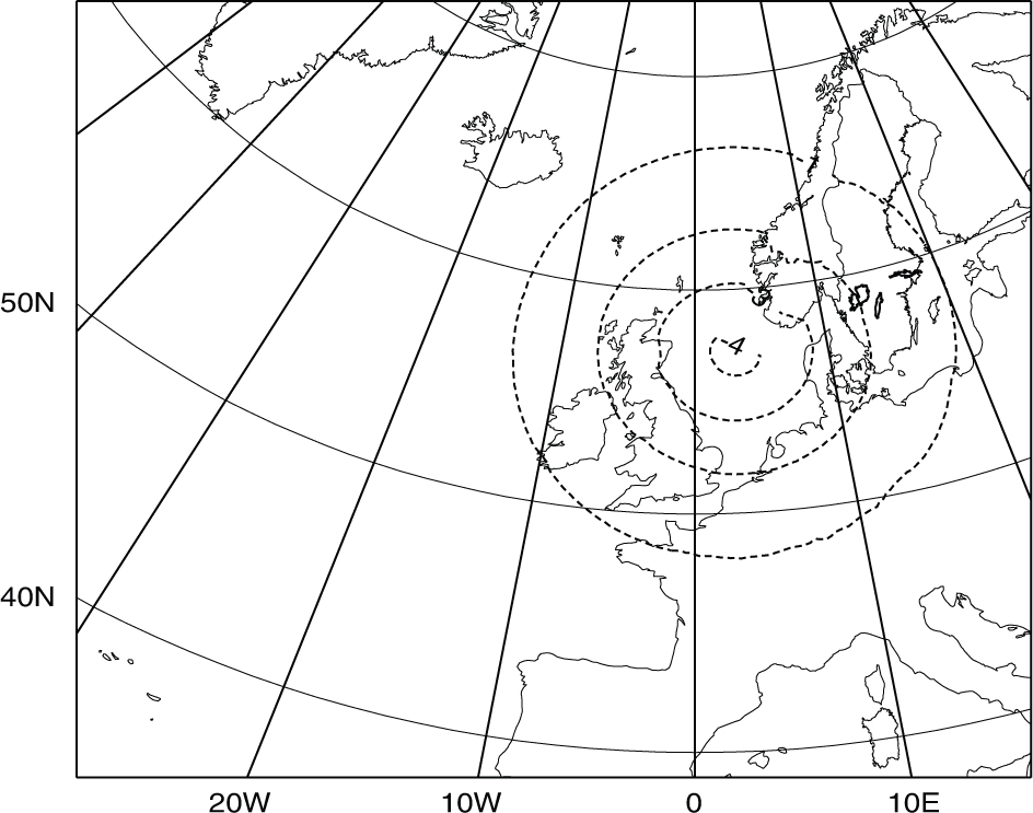
Fig. 3.
4D-Var surface pressure assimilation increments for 3 December 1999, 11 UTC, from a single surface pressure observation increment of −5 hPa at 57°N 3°E for 3 December 1999, 11 UTC. The data assimilation window is from 06 UTC until 12 UTC. The assumed standard deviation of the observation error is 0.5 hPa. The contour interval is 1 hPa.
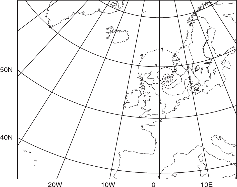
Fig. 4.
Vertical cross-section with 4D-Var assimilation increments of temperature and the wind component normal to the vertical cross-section at 3 December 1999, 06 UTC, from a single surface pressure observation increment of −5 hPa at 57°N 3°E with observation time 3 December 1999, 11 UTC. The data assimilation window is from 06 UTC until 12 UTC. The assumed standard deviation of the observation error is 0.5 hPa. The vertical cross-section extends from 67°N 25°W until 48°N 15°E. Contour intervals are 0.5 m s−1 and 0.1 K.
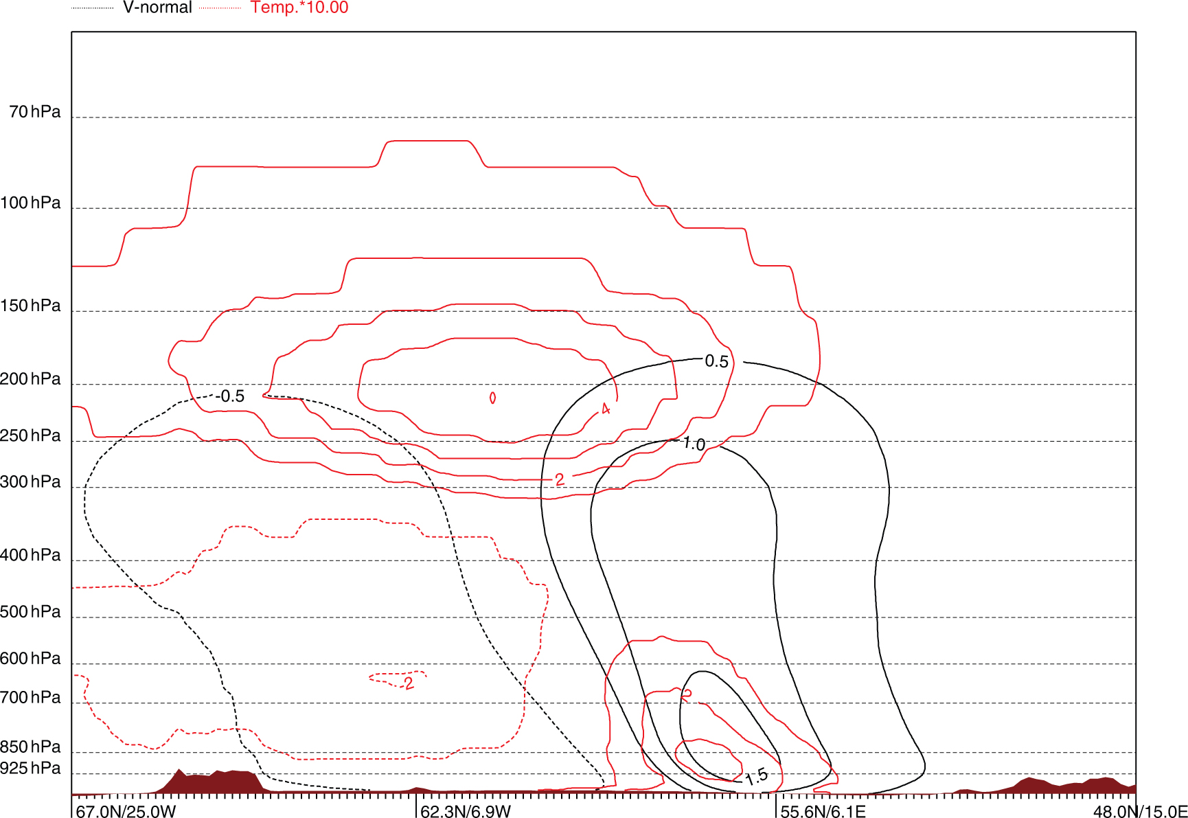
Fig. 5.
4D-Var surface pressure assimilation increments for 3 December 1999, 11 UTC, from a single surface pressure observation increment of −5 hPa at 55°N 20°W for 3 December 1999, 11 UTC. The data assimilation window is from 06 UTC until 12 UTC. The assumed standard deviation of the observation error is 0.5 hPa. The contour interval is 1 hPa.
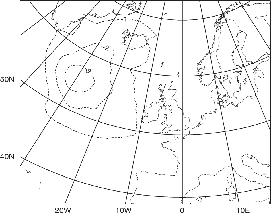
Fig. 6.
The HIgh Resolution Limited Area Model RCR data assimilation and forecast domain.
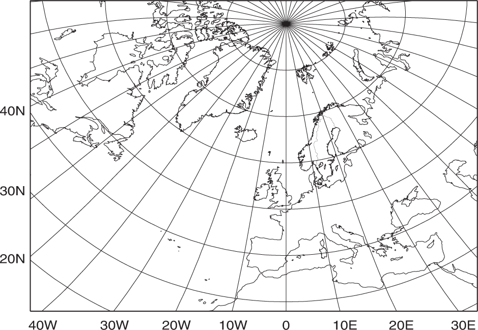
Fig. 7.
The observation contribution J o (a) and the normalised digital filter constraint contribution (b) to the total cost function as a function of the inner loop minimisation iteration number for different values of the weak digital filter constraint coefficient =0.001, 1.0, 4.0, 16.0 and 32.0. First outer loop iteration with 50 inner loop minimisation iterations for a horizontal increment resolution of 6× the non-linear model resolution. The RCR domain with 60 levels and 16 km horizontal resolution is applied in the non-linear model.
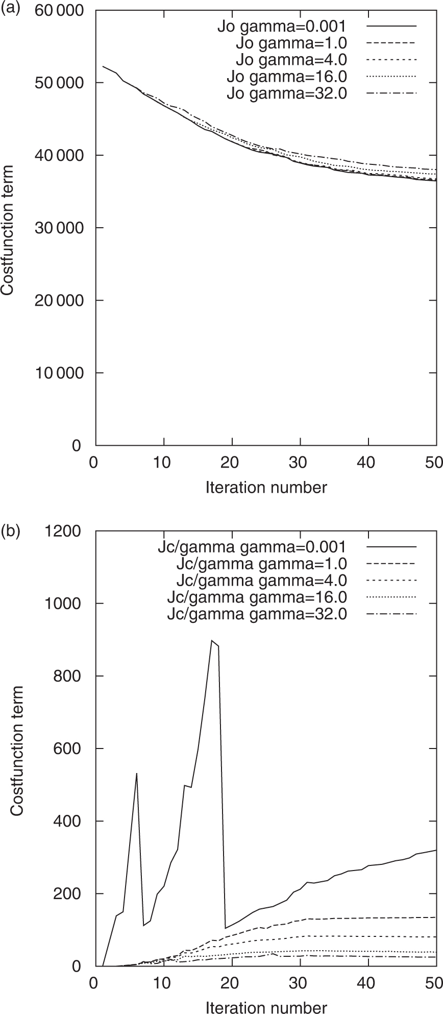
Fig. 8.
Horizontal average of the absolute value of the surface pressure tendency (in hPa/3 h) for every time-step, with a time step length of 6 minutes, during the non-linear model integration over 5 h from initial data based on HIgh Resolution Limited Area Model 4D-Var, including a weak digital filter constraint with different values of the weak digital filter constraint coefficient =0.001, 1.0, 4.0, 16.0 and 32.0. One outer loop iteration with 50 inner loop minimisation iterations for a horizontal increment resolution of 6× the non-linear model resolution and the RCR domain with 60 levels and 16 km horizontal resolution in the non-linear model are applied.
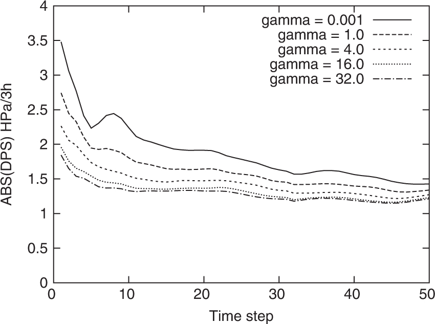
Fig. 9.
The observation error constraint contribution J o (a) and the background error constraint contribution J b (b) to the total cost function as a function of the total inner loop minimisation iteration number for four different minimisation strategies: (1) one outer loop minimisation with a 48 km horizontal resolution of the assimilation increment and with 100 inner loop iterations; (2) two outer loop iterations, both with 50 iterations in the inner loops and with 48 km resolution of the increments; (3) and (4) two experiments with two outer loop iterations, both with 96 km resolution in the first outer loop and with 48 km in the second outer loop, one experiment with 30 inner loop iterations in the first outer loop and with 70 iterations in the second outer loop. Another experiment has 60 iterations in the first outer loop and 40 iterations in the second outer loop. The RCR domain with 60 levels and 16 km horizontal resolution in the non-linear model is applied.
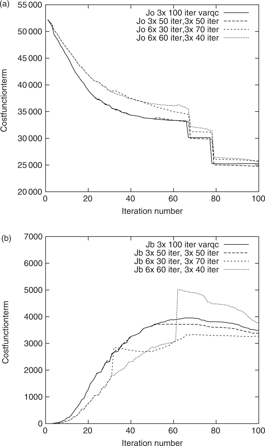
Fig. 10.
Kinetic energy spectrum at model level 30 (around 500 hPa) for the assimilation increments. (a) After 10, 20, 30, 50 and 100 inner loop iterations of a 4D-Var minimisation with a single outer loop iteration with a 48 km horizontal resolution of the increments. (b) Same as in (a) but for the experiment with two outer loop iterations, with 60 iterations at 96 km resolution in the first outer loop and with 40 iterations at 48 km in the second. The assimilation was carried out with the HIgh Resolution Limited Area Model 4D-Var for the RCR domain with 60 levels and 16 km horizontal resolution in the non-linear model.
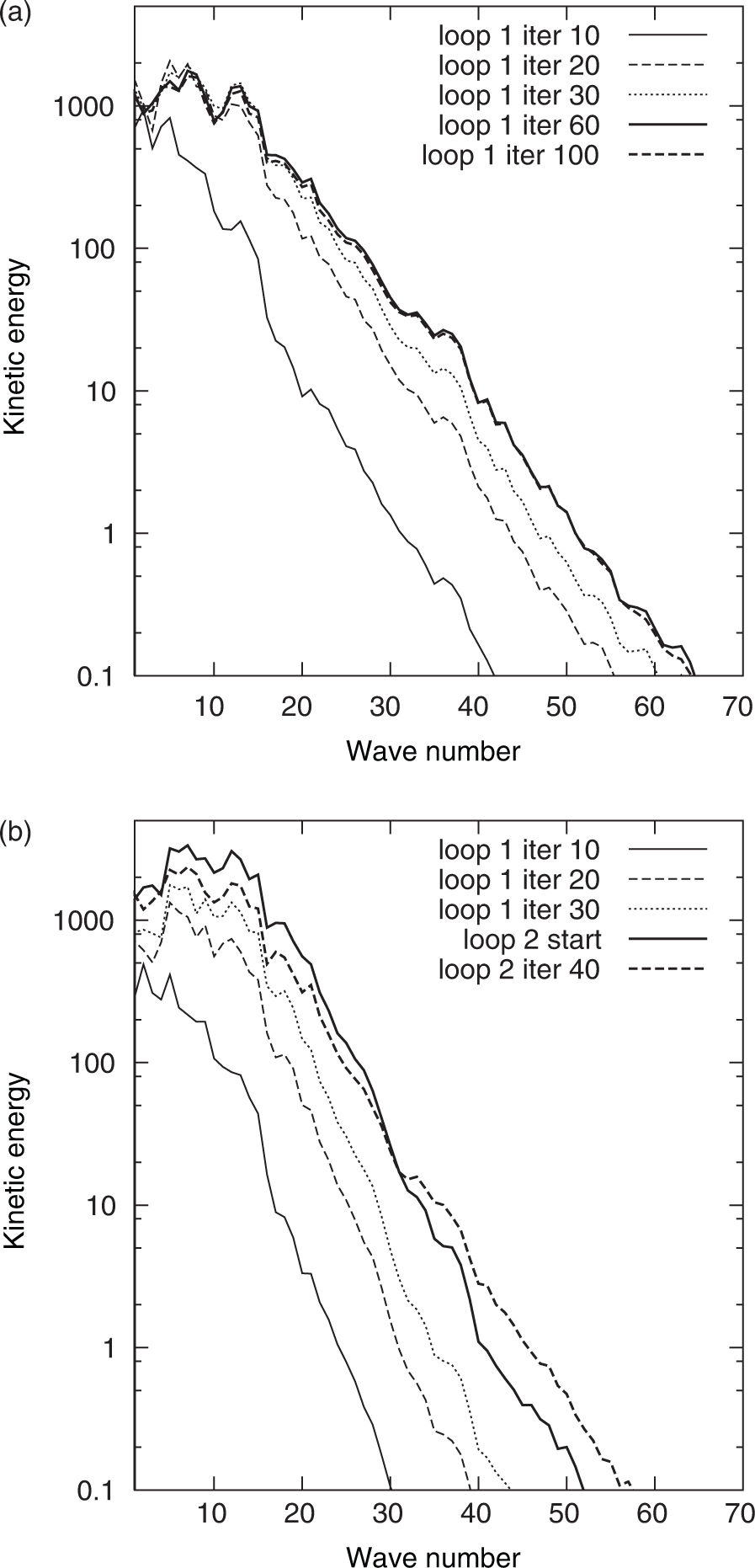
Fig. 11.
BIAS (mean error, thin lines) and root mean square error (RMSE, thick lines) mean sea level pressure (MSLP) verification scores for June 2005 as a function of forecast length. Verification against surface observations over a Scandinavian domain. Experiment 4DVAR1 (full lines): 4D-Var with one outer loop iteration at 66 km resolution, experiment 4djun05D (dashed lines): 4DVAR with one outer loop iteration at 44 km resolution and experiment 4DVAR2 (dotted lines): 4DVAR with two outer loop iterations at 66 km and 44 km resolution, respectively.
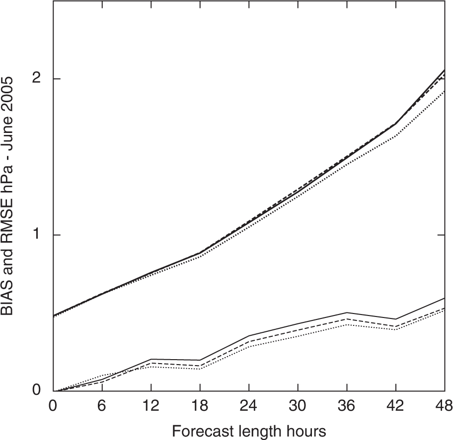
Table 1. Numbers of Active Observed Values that Enter the 3D-Var and 4D-Var Minimisations for 12 January 2007 06 UTC (a) and 12 UTC (b)
Fig. 12.
BIAS (Mean error, thin lines) and root mean square error (RMSE, thick lines) mean sea level pressure (MSLP) forecast verification scores for a Scandinavian domain as a function of forecast length. Time averaged scores for April 2004 (a), January 2005 (b), June 2005 (c) and January 2007 (d). 3D-Var (full line), 4D-Var with one outer loop iteration (dashed line) and 4D-Var with two outer loop iterations (dotted lines).
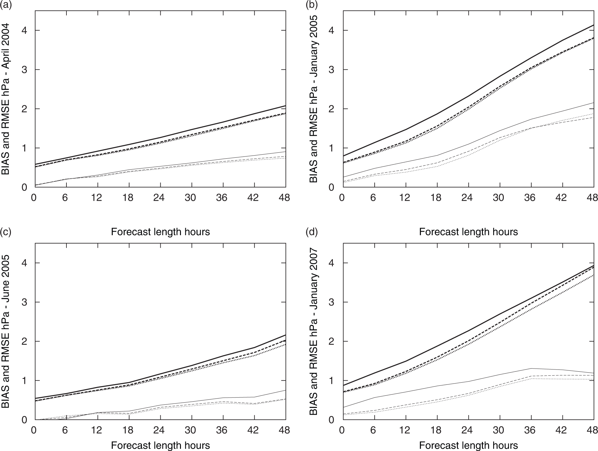
Fig. 13.
Normalised mean root mean square error (RMSE) forecast verification score differences (green curves) between 3D-Var and 4D-Var (with one outer loop iteration) for mean sea level pressure (MSLP) over a European domain as a function of forecast length. Time-averaged scores for April 2004 (a), January 2005 (b), June 2005 (c) and January 2007 (d). Vertical red bars represent significance at the 90% level.
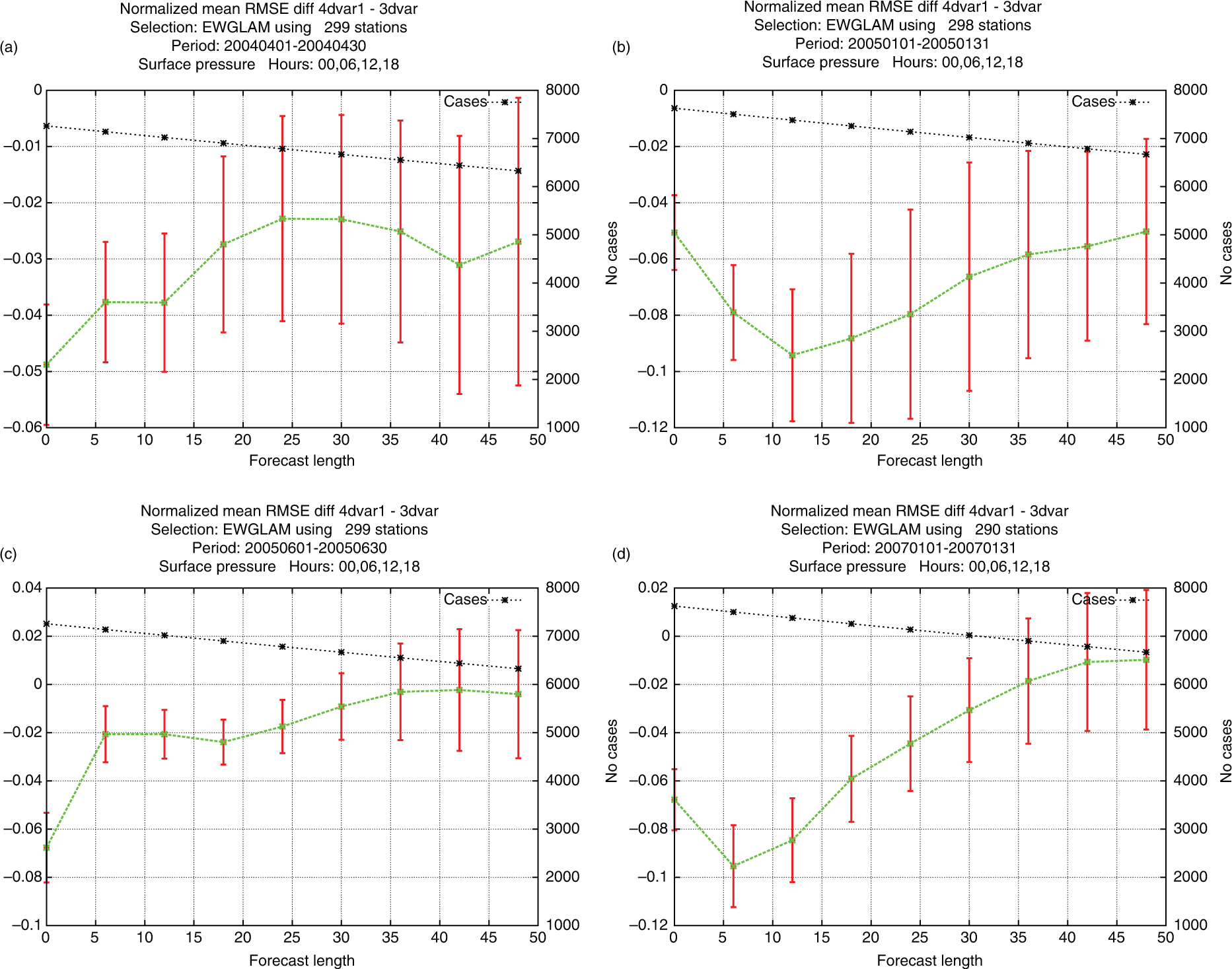
Fig. 14.
HIgh Resolution Limited Area Model 4D-Var mean sea level pressure (MSLP) analysis for 3 December 1999, 18UTC. The contour interval is 2 hPa.
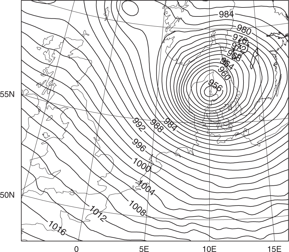
Fig. 15.
HIgh Resolution Limited Area Model 4D-Var mean sea level pressure analysis for 27 December 1999, 18 UTC. The contour interval is 2 hPa.
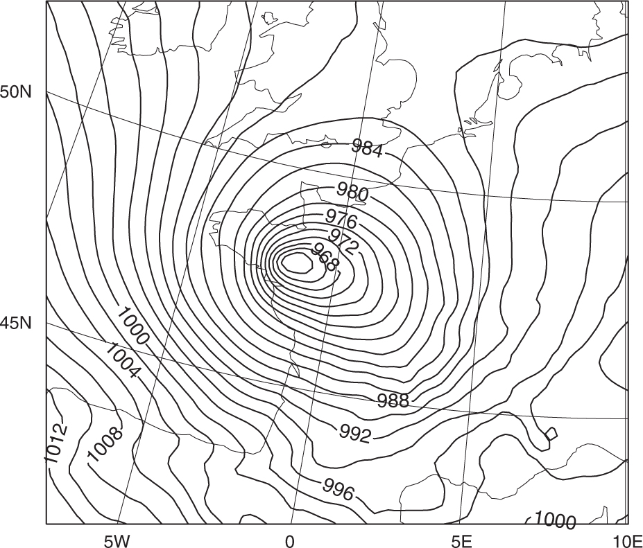
Fig. 16.
BIAS (mean error, thin lines) and root mean square error (RMSE, thick lines) mean sea level pressure (MSLP) forecast verification scores for a European domain as a function of forecast length. Time averaged scores for December 1999. 3D-Var (full lines) and 4D-Var (dashed lines).
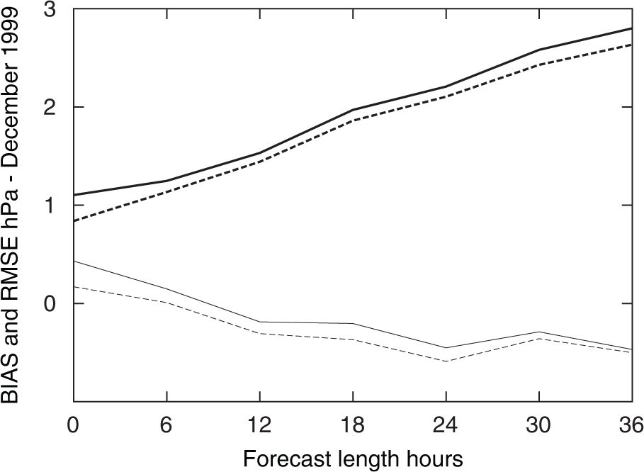
Fig. 17.
+30 h mean sea level pressure (MSLP) forecasts valid at 3 December 1999, 18 UTC, based on 3D-Var (a) and 4D-Var (b) initial data from 2 December 1999, 12 UTC. The contour interval is 2 hPa.
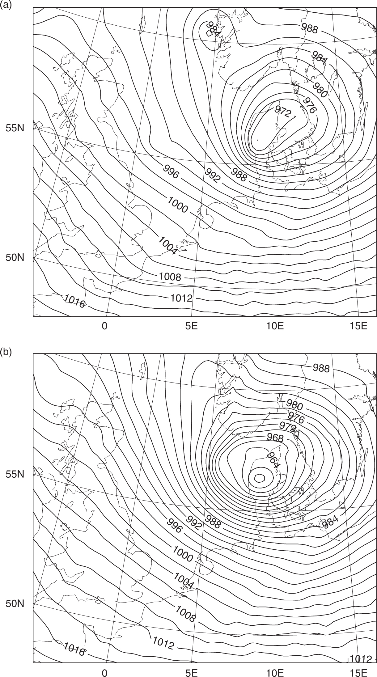
Fig. 18.
+18 h mean sea level pressure (MSLP) forecasts valid at 3 December 1999, 18 UTC, based on 3D-Var (a) and 4D-Var (b) initial data from 3 December 1999, 00 UTC. The contour interval is 2 hPa.
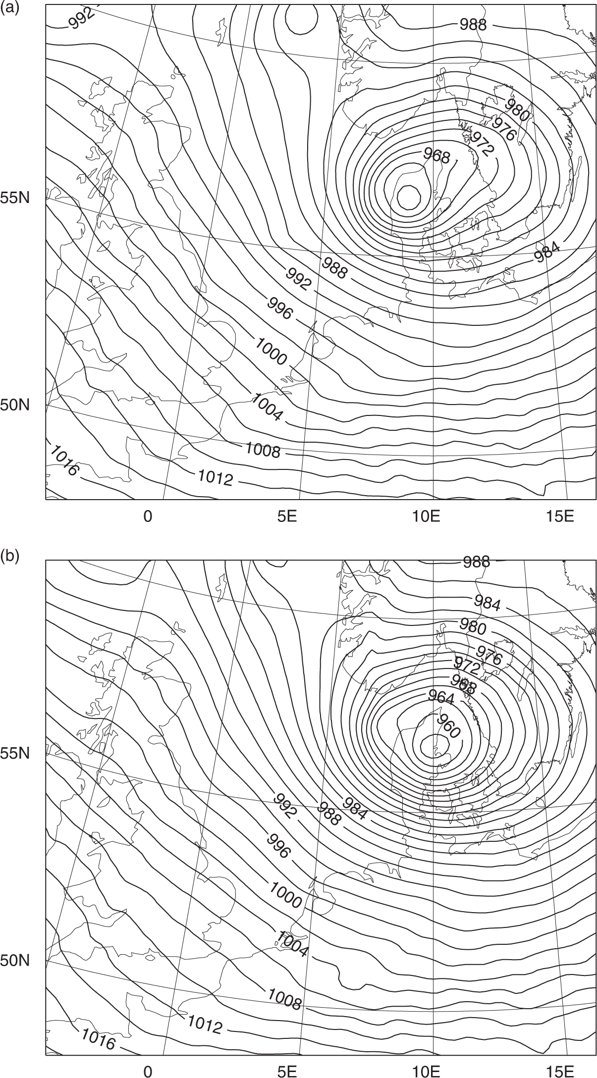
Fig. 19.
Surface pressure assimilation increments for 3 December 1999, 06 UTC, with 3D-Var (a) and with 4D-Var (b). The contour interval is 1 hPa.
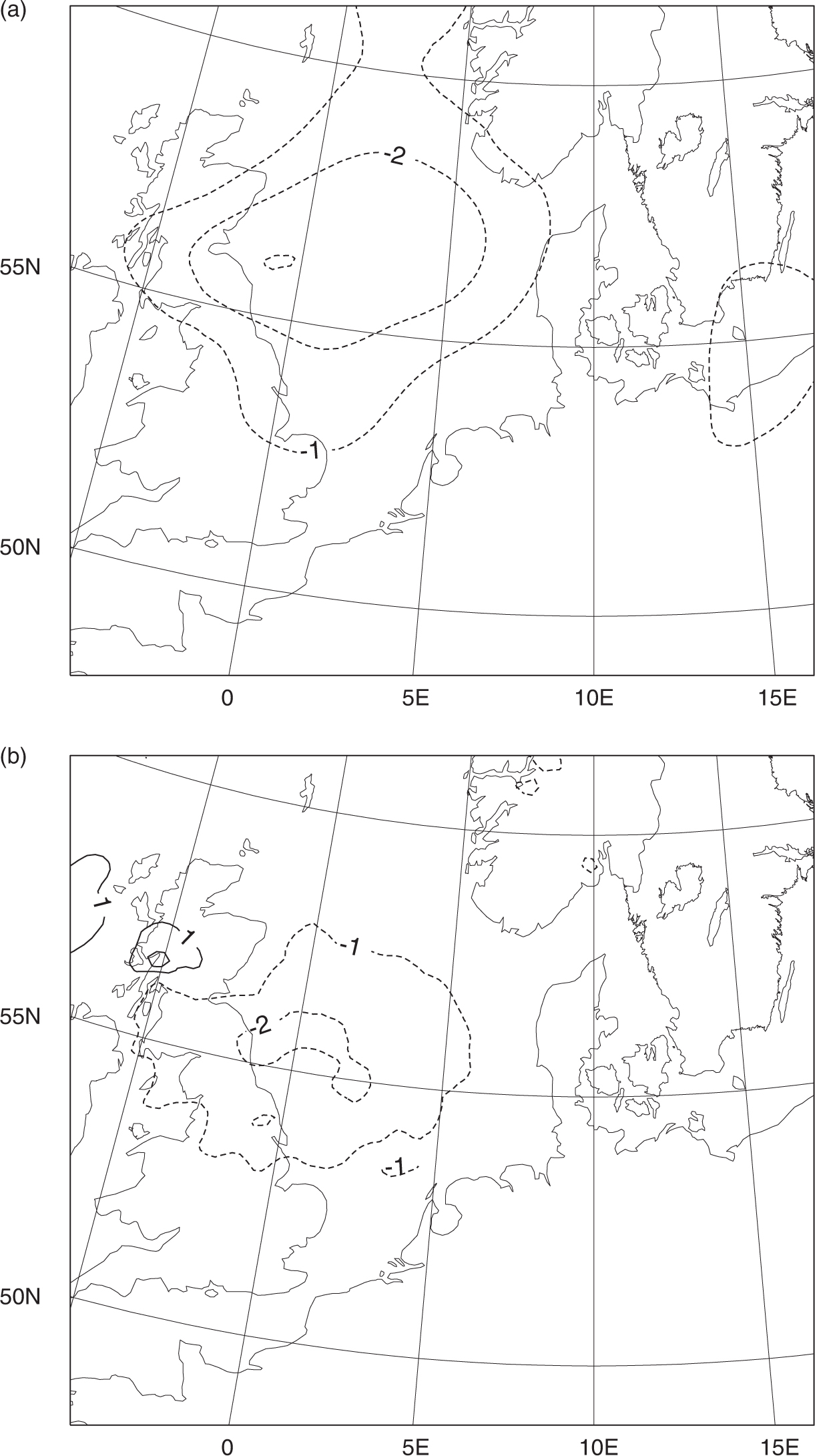
Fig. 20.
Surface pressure assimilation increments for 3 December 1999, 12UTC, with 3D-Var (a) and with 4D-Var (b). The contour interval is 1 hPa.
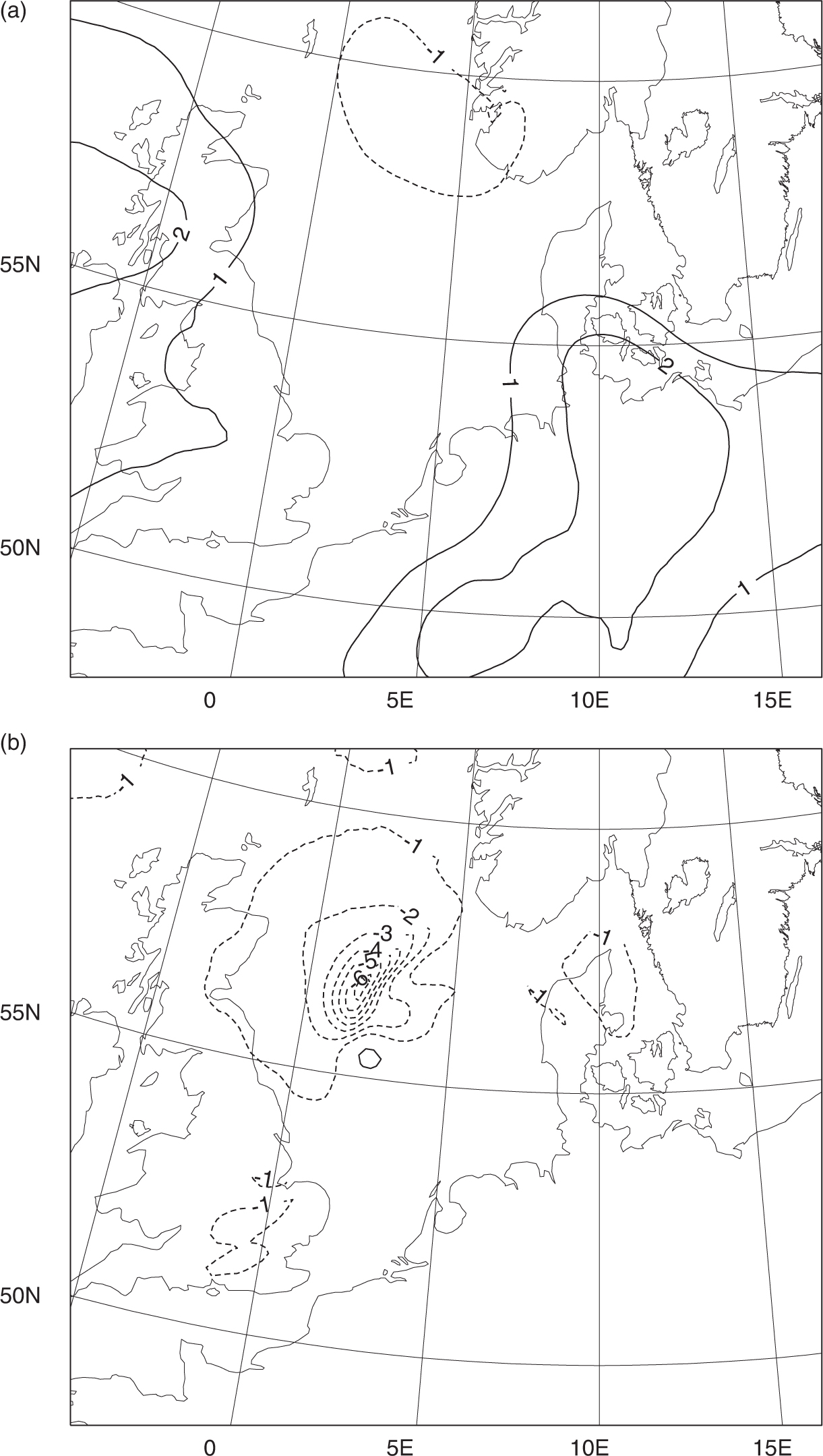
Fig. 21.
+6 h mean sea level pressure (MSLP) forecasts valid at 27 December 1999, 18 UTC, based on 3D-Var (a) and 4D-Var (b) initial data at 27 December 1999, 12 UTC. The contour interval is 2 hPa.
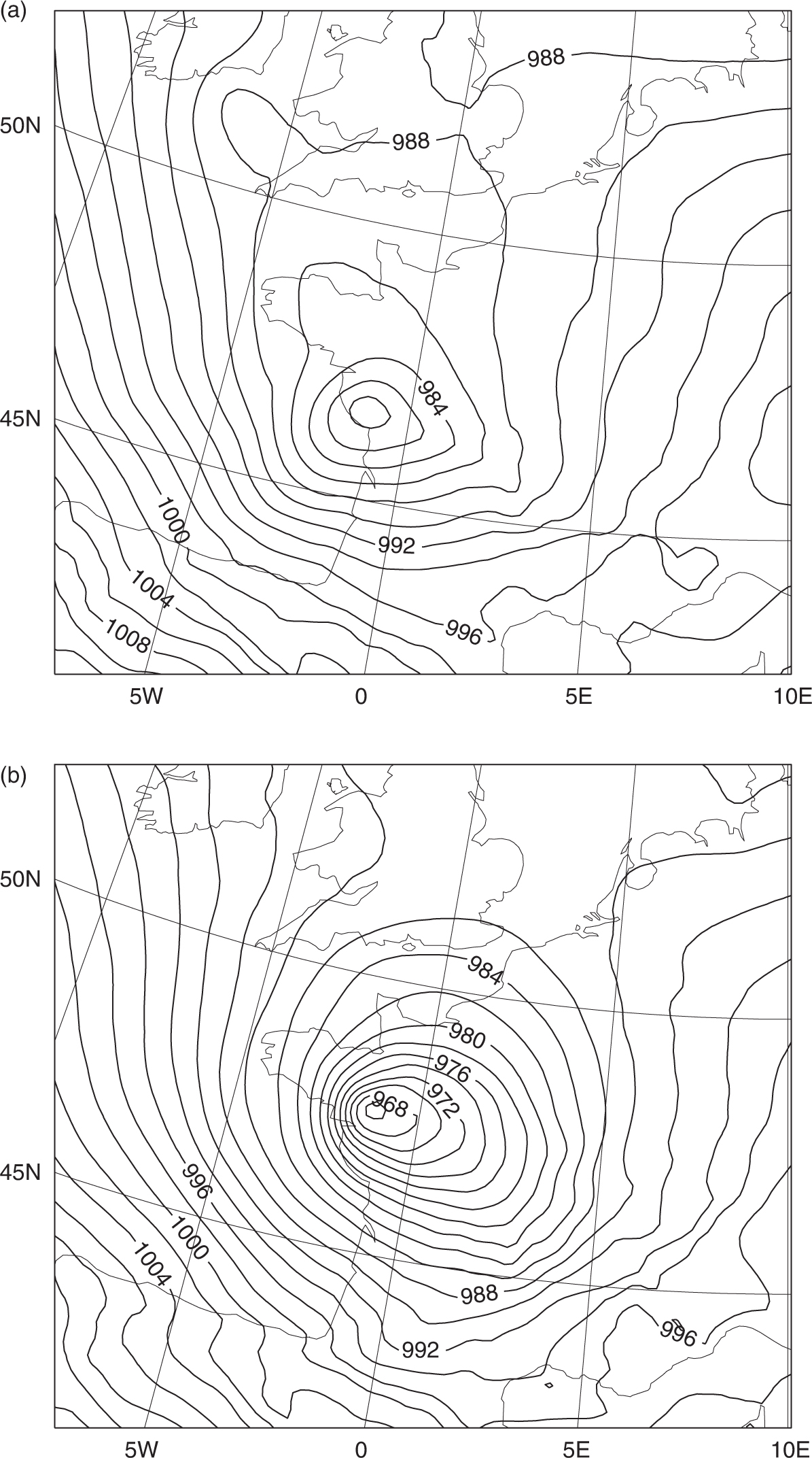
Table 2. Example of Computation Times in Seconds on an IBM Computer with 32 Processors for Different parts of HIRLAM 4D-Var
[i] (a) 30 inner loop iterations at 96 km increment resolution; (b) 40 inner loop iterations at 48 km increment resolution, both with 60 vertical levels. The non-linear model domain is the RCR with a 16 km horizontal resolution.