
Fig. 1.
(a) Best track; and (b) minimum sea level pressure (SLP, hPa) of TC Sinlaku (200813) from the Regional Specialised Meteorological Centre (RSMC) Tokyo. The shaded area in (b) represents the period of time over which the data assimilation was performed.
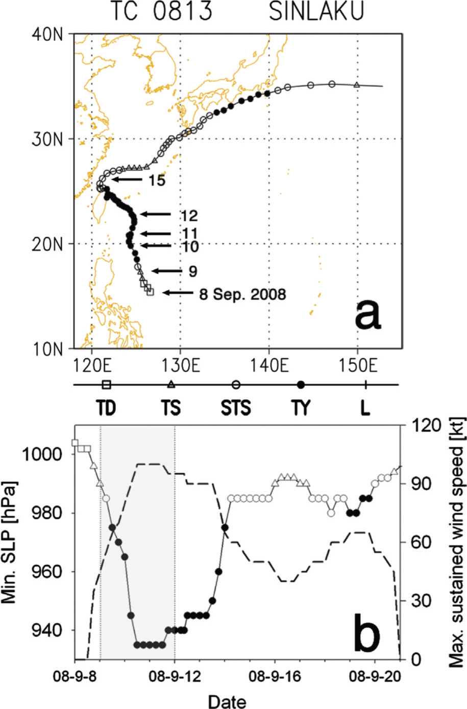
Fig. 2.
SLP (thin lines at 4 hPa intervals) and geopotential height (thick lines at intervals of 60 gpm) on 500 hPa of NCEP FNL at: (a) 1200 UTC 9; (b) 1200 UTC 10; and (d) 0000 UTC 14 September 2008. The shaded area denotes the subtropical ridge (over 5880 gpm), and the thick arrows indicate the translational velocity of TC Sinlaku. The radar reflectivity (shaded, at 5 dBZ intervals) from the Central Weather Bureau (CWB) of Taiwan for 1600 UTC 13 September 2008 is shown in (c).
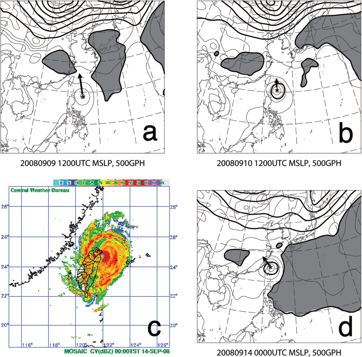
Table 1. Multiple physics configuration for the ensembles
Fig. 3.
Observational distribution for: (a) surface observations (red cross for station [SYNOP], blue dot for buoy, and green dot for ship); (b) upper air observations (blue dot for radiosonde and red dot for targeted dropsonde); (c) aircraft observations (blue cross) and position of best track (orange star); and (d) AMV from MTSAT (blue, red, and green for upper-, mid- and lower-troposphere, respectively) at 0000 UTC 10 September 2008. The SLP (solid lines at 4 hPa intervals) of NCEP FNL are superposed on (a) and (b).
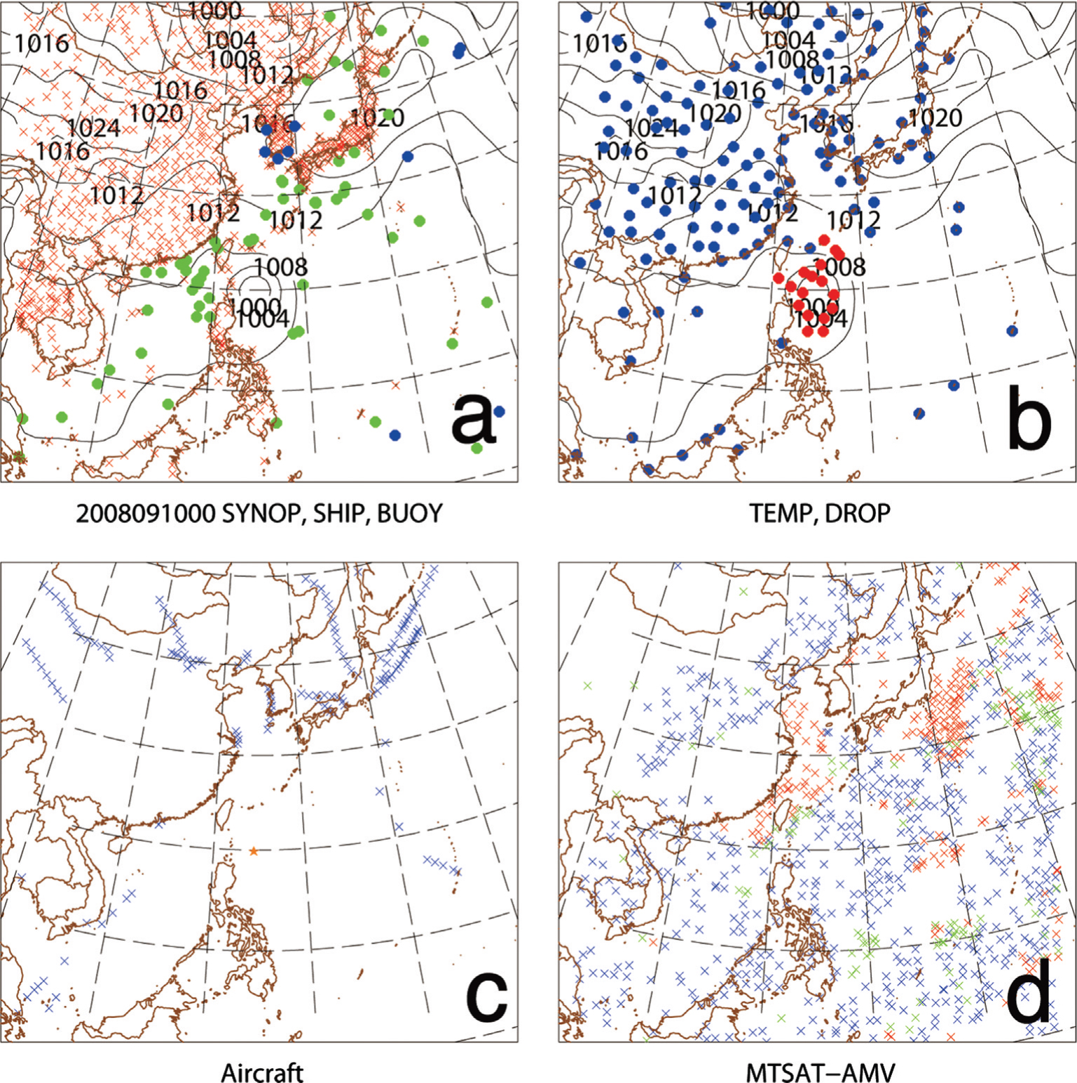
Fig. 4.
Distribution of targeted dropsonde observations superposed with SLP (solid lines at 4 hPa intervals) of NCEP FNL at: (a) 0600 UTC 9; (b) 0000 UTC 10; (c) 0600 UTC 10; (d) 0000 UTC 11; (e) 0600 UTC 11; and (f) 1200 UTC 11 September 2008. The red dot represents observations within 100 km of the typhoon centre.
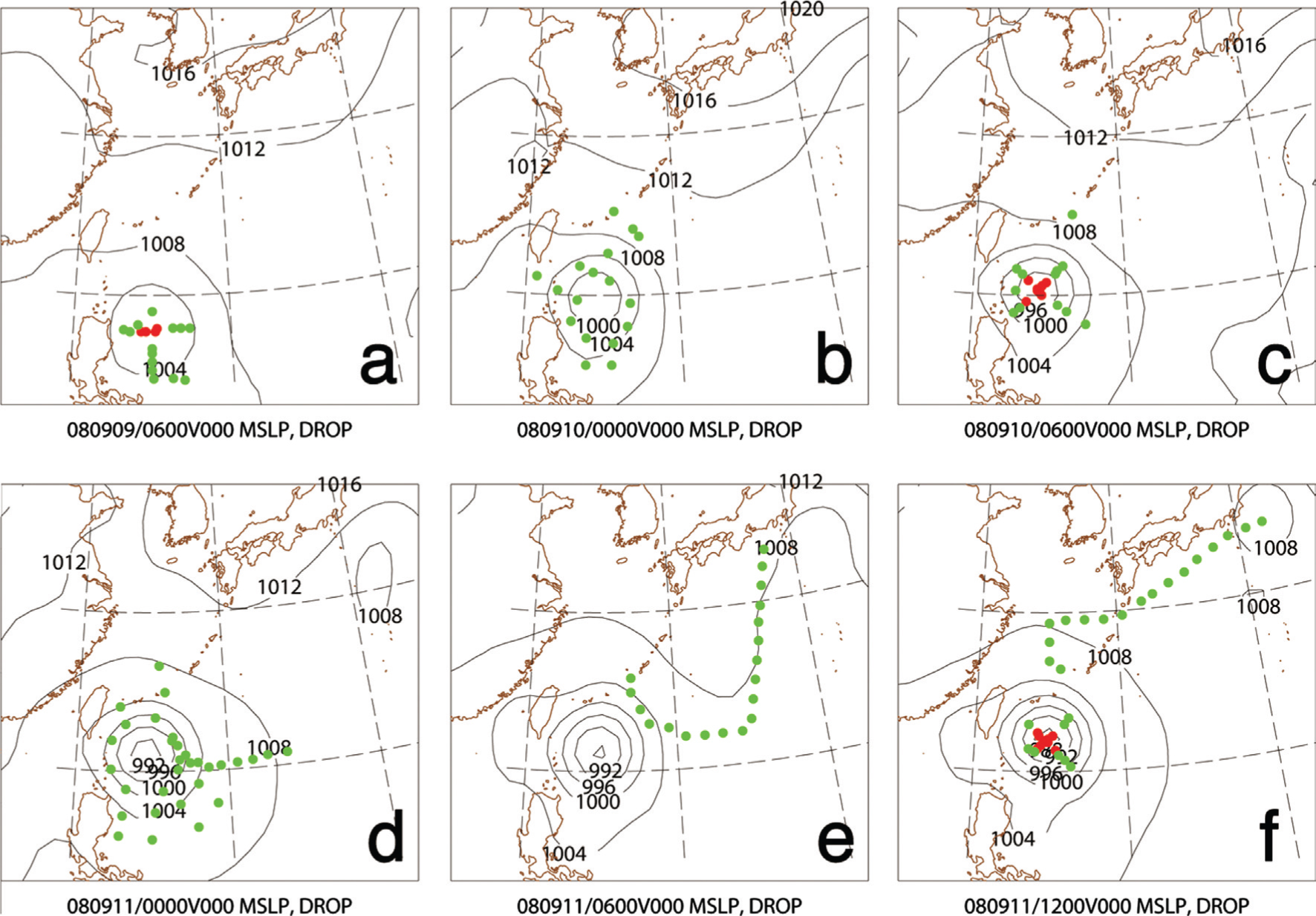
Table 2. Description of numerical experiments
Fig. 5.
The RMSE (solid lines), spread (dotted lines), bias (dashed lines) of prior (blue colored lines) and posterior (red colored lines) ensemble-mean fields accumulated for all analysis times for: (a) U; (b) V; (c) T; and (d) Q components, verified via radiosonde and dropsonde observations in the mandatory levels. The observational error for each observational variable is denoted by a green line with cross marks, and the predicted RMSE is denoted by a blue line with closed circles.
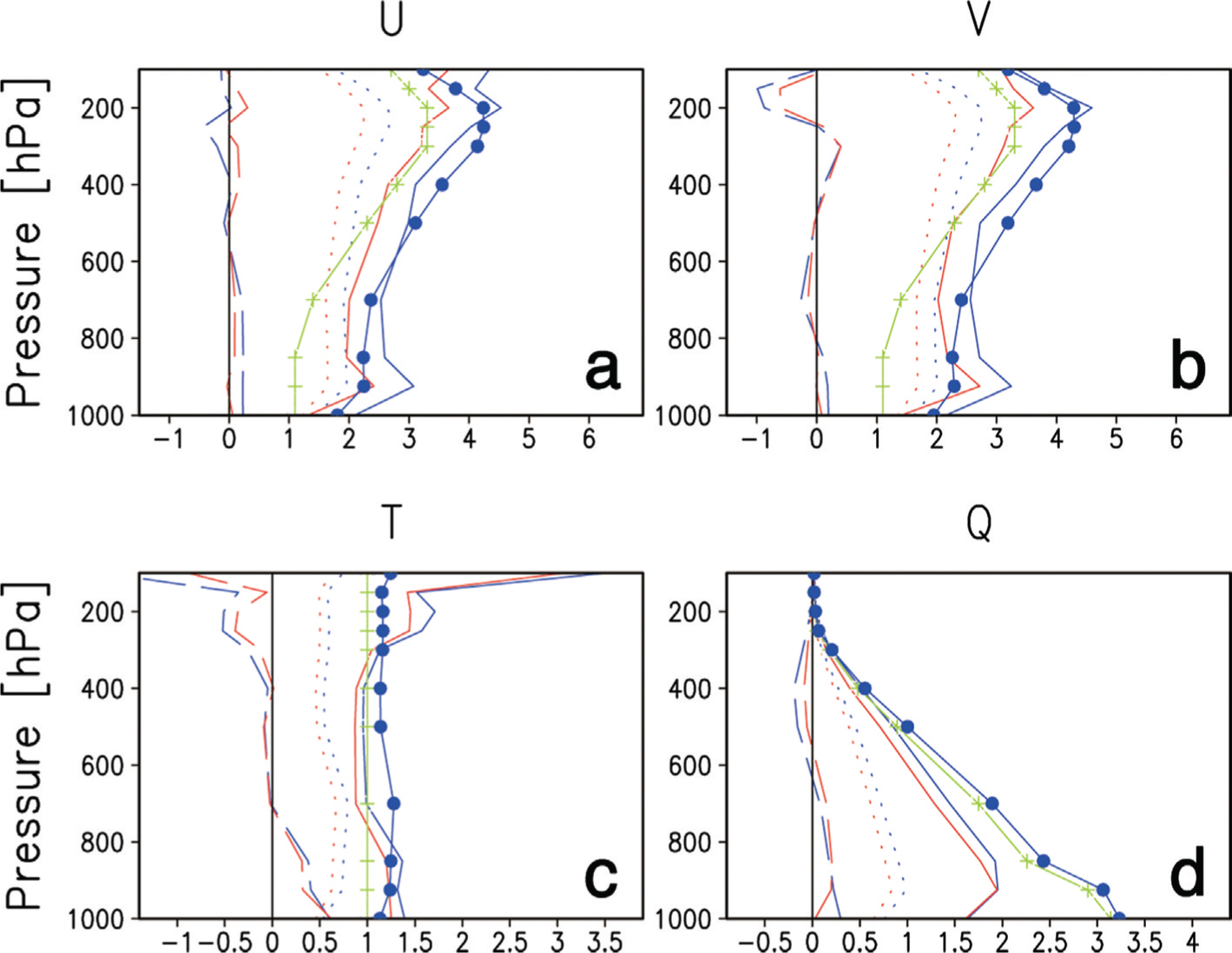
Fig. 6.
Rank histograms of prior ensembles accumulated for all analysis times for: (a, e) U; (b, f) V; (c, g) T; and (d, h) Q components, verified via radiosonde and dropsonde observations in the mandatory levels. The observational error is incorporated into the rank histograms in the lower panels (e–h). The dashed black lines denote the ideal value for the rank histograms (e.g., 100/37 = 2.70).
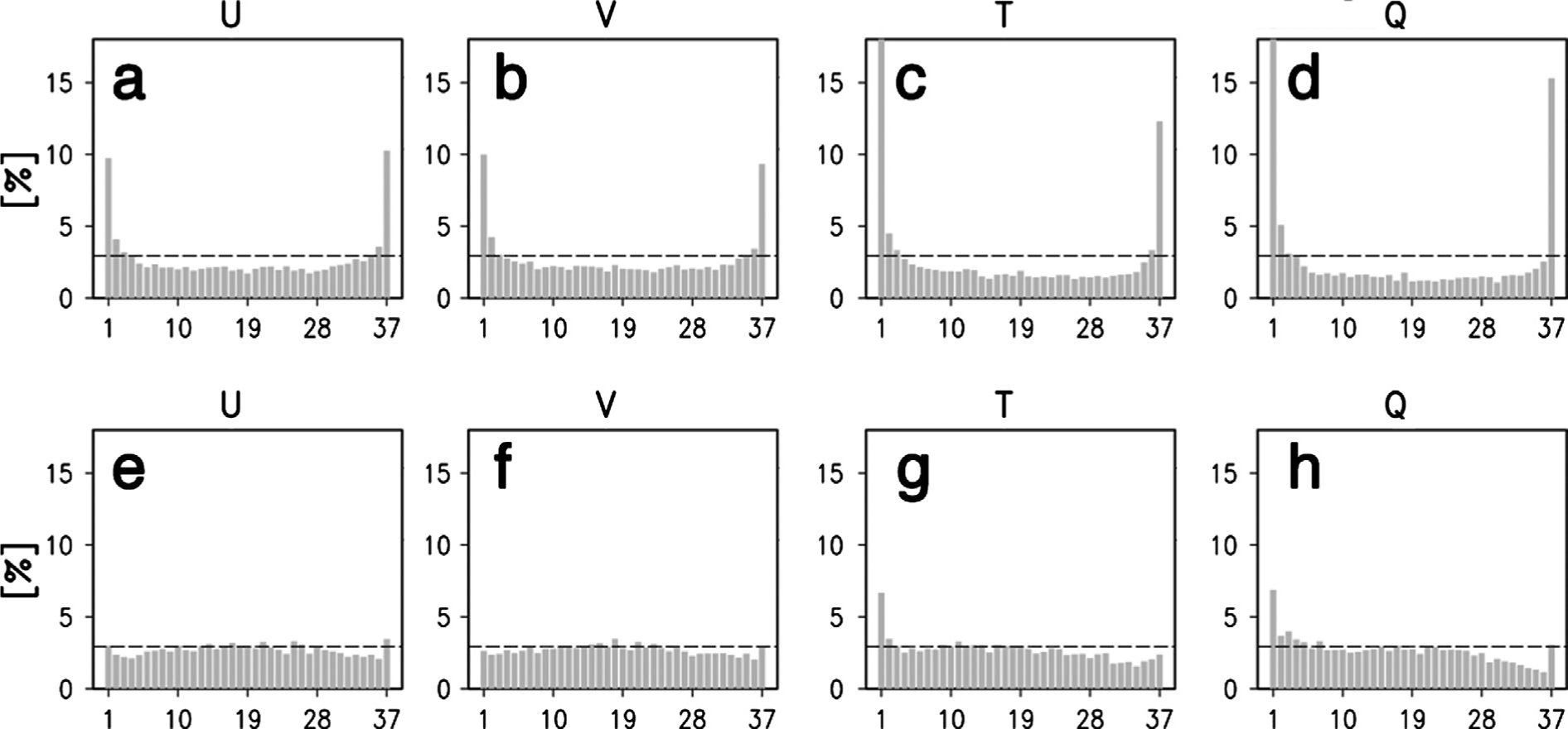
Fig. 7.
The ensemble-mean SLP (solid lines at 4 hPa intervals) and corresponding spread (shaded region, hPa) of (a) prior and (b) posterior ensembles for domain 1 of EXP2 at 0000 UTC 11 September 2008, those of (c) prior and (d) posterior ensembles for domain 2 of EXP2, and those of (e) prior and (f) posterior ensembles for domain 1 of EXP4. The SLP of 1000 hPa is denoted by a thick solid line, and the best track position is indicated by a solid black dot in each figure.
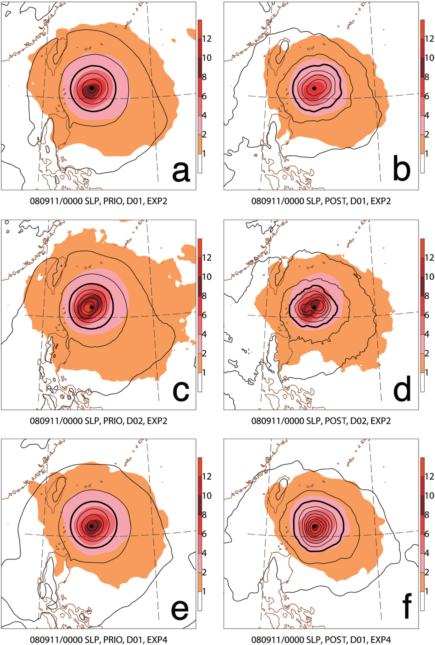
Fig. 8.
Ensemble-mean tracks for domain 1 (upper panels) and domain 2 (lower panels) initiated at: (a, d) 0000 UTC 10; (b, e) 0000 UTC 11; and (c, f) 0000 UTC 12 September 2008. The lines represent the best track (thick black line), EXP1 (thin black line), EXP2 (red line), EXP3 (green line), EXP4 (blue line), EXP5 (orange line), and CORE (yellow line), respectively.
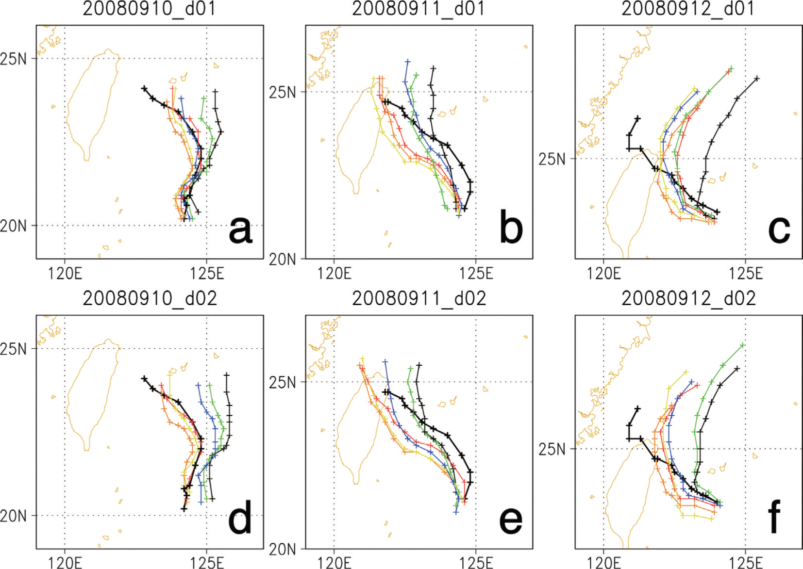
Fig. 9.
Seventy two-hour averaged forecast errors (km) of ensemble-mean tracks for the indicated experiments initiated at: (a) 0000 UTC 10; (b) 0000 UTC 11; and (c) 0000 UTC 12 September 2008.
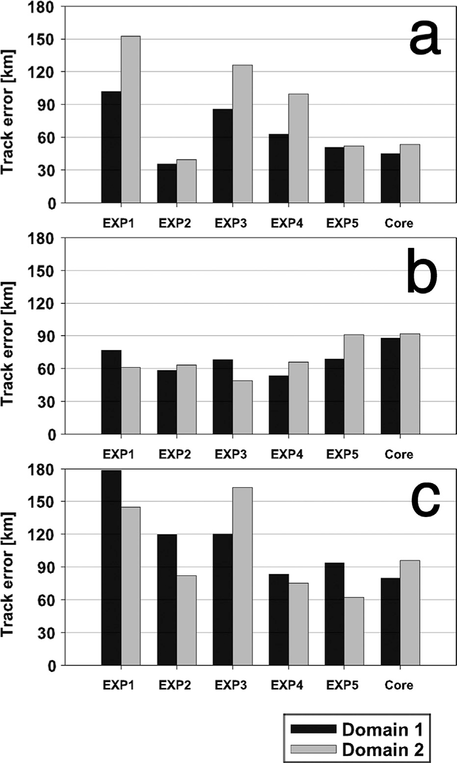
Table 3. Differences (upper and left experiment) of time-averaged track errors between the major experiments shown in Fig. 9
[i] The bold (italic) numbers are within the 95% (90%) confidence interval, after implementing the paired t-test.
Fig. 10.
Seventy two-hour averaged RMSE of ensemble-mean forecast fields for experiments initiated at: (a) 0000 UTC 10; (b) 0000 UTC 11; and (c) 0000 UTC 12 September 2008. The forecast fields are verified with radiosonde and dropsonde observations in the mandatory levels. The units for T, U, V, Q, and RM-DTE are K, m s−1, m s−1, g kg−1 and m s−1, respectively.
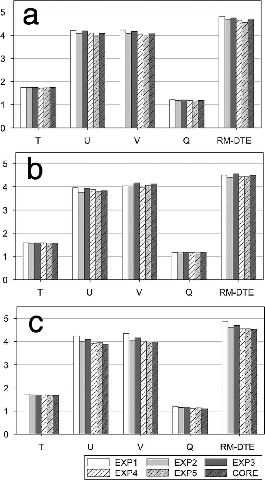
Table 4. The rejection rate (%), total number of observations, and number of corresponding soundings of dropsonde observations for six analysis times (see Fig. 4)