Fig. 1.
Schematic diagrams of (a) the MBD method and (b) the LET method.

Table 1. List of data assimilated in the Meso 4D-VAR and LETKF analyses
Fig. 2.
Schematic diagram of the preparation procedure for LBCs and LBPs.
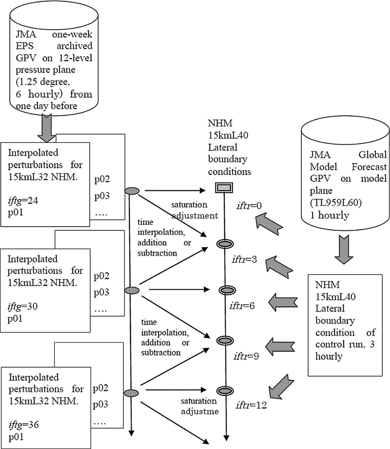
Fig. 3.
Time sequence of the statistical ensemble spread of the 500 hPa height filed in the JMA's global one-week EPS. A line indicated by triangles is the spread by the global BGM before October 2007, whereas squares indicate the spread by the global SV method after November 2007. Courtesy of Ryouta Sakai of JMA.
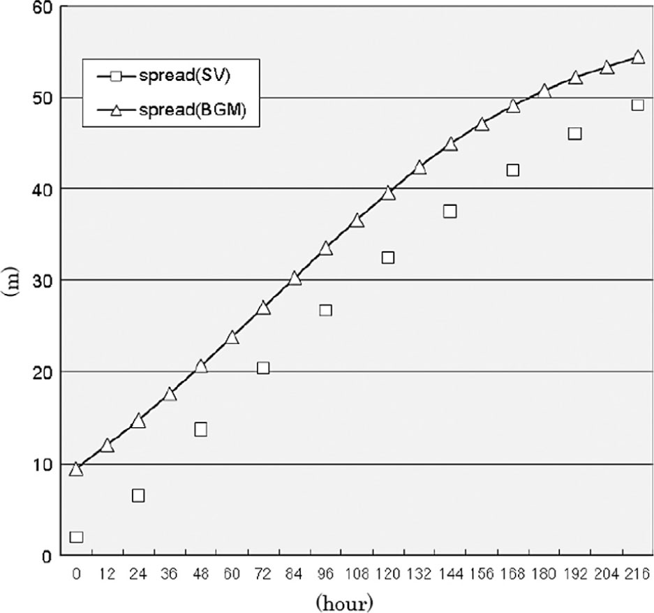
Fig. 4.
Sea level pressure (contours) and accumulated 3-h precipitation (colour scale) predicted by the control run. Initial time is 12 UTC, 4 July 2008. The colour bar indicates precipitation intensity in mm. (a) FT=3. (b) FT=24.
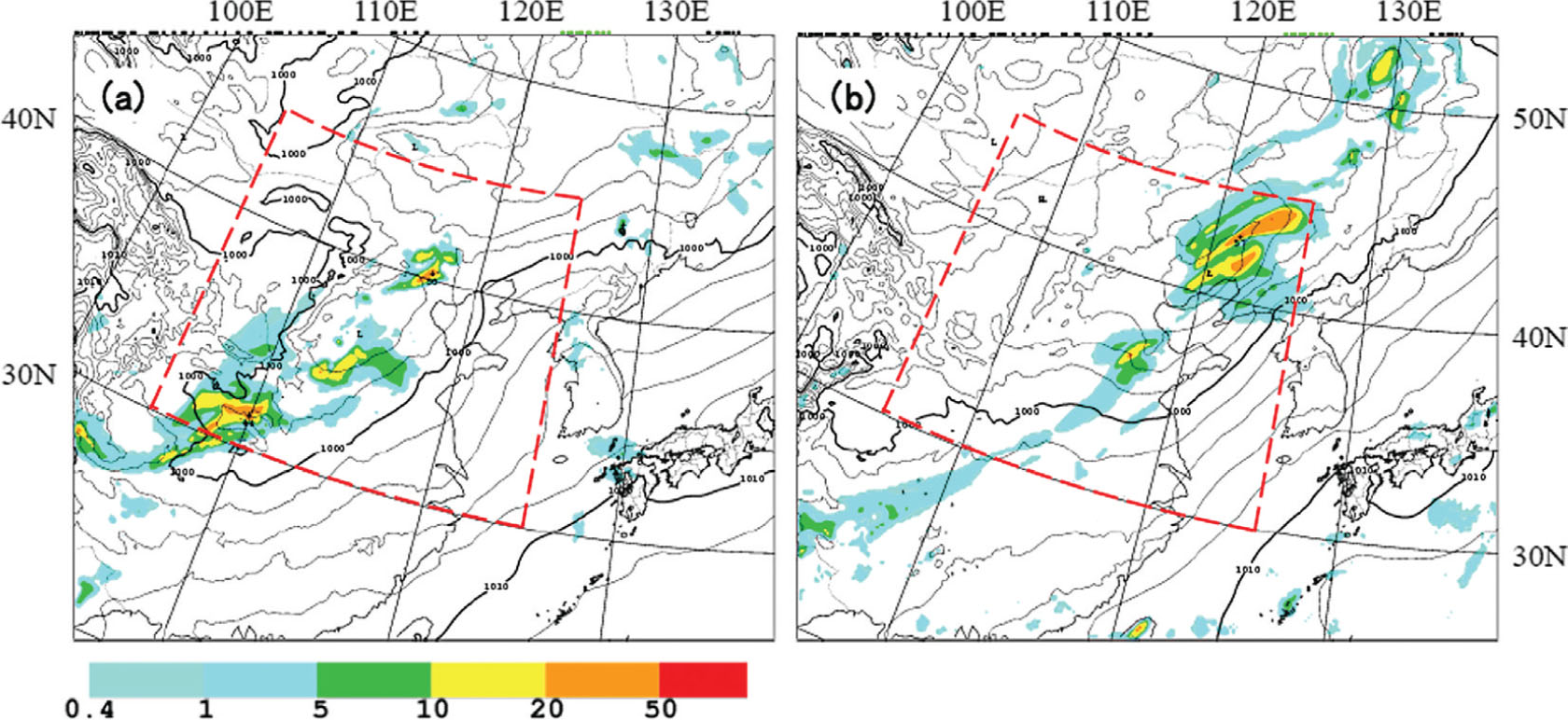
Table 2. List of experiments
Fig. 5.
(a) Ensemble spread for meridional horizontal wind (V) at 850 hPa in the experiment with LBP only (NIP_lbpf). Initial time is 12 UTC 4 July 2008. (b) Ensemble spread at FT=36. (c) Time sequence of the ensemble spreads of surface elements in the common verification area.
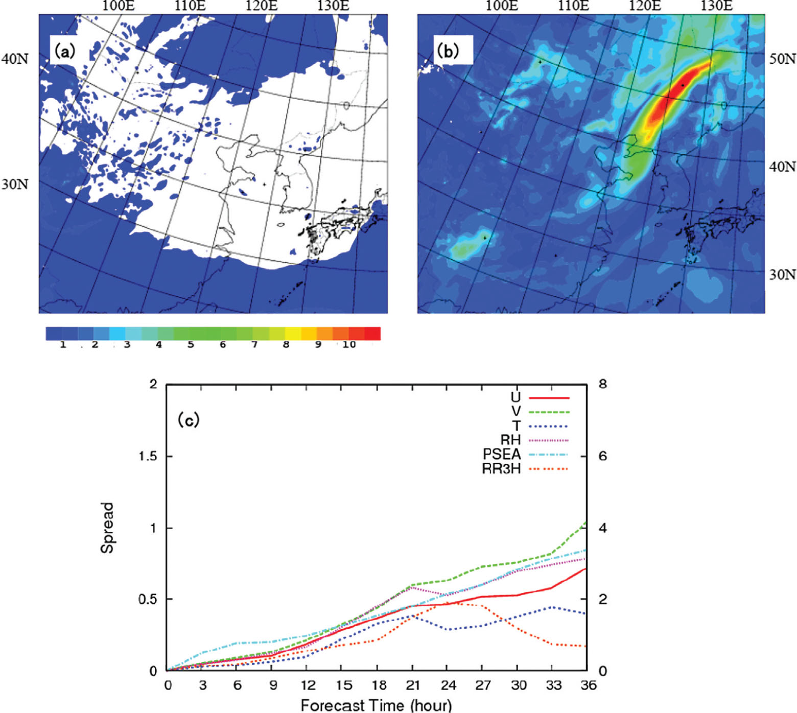
Fig. 6.
Similar to Fig. 5 but for the MBD experiment without LBPs (MBD_nlbp).
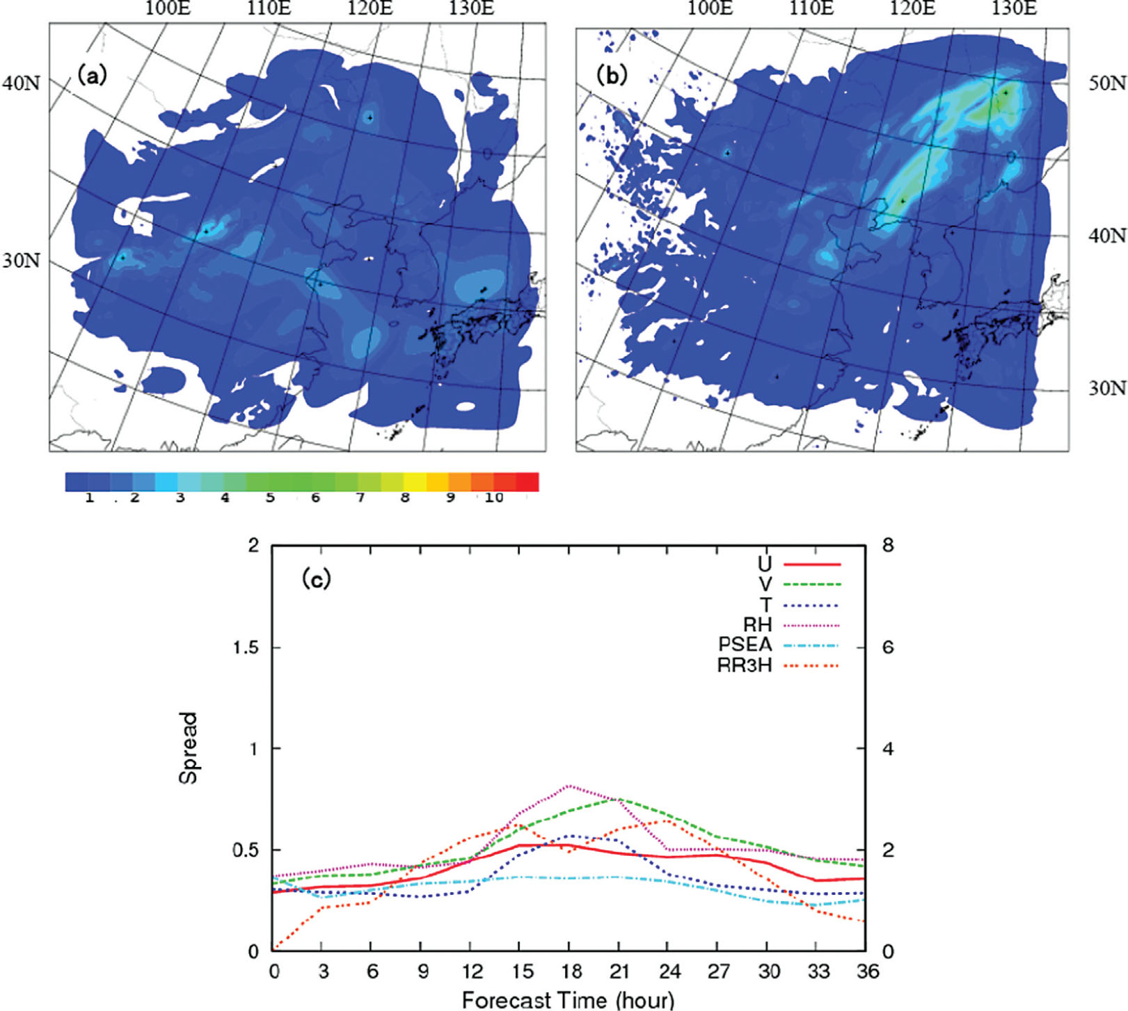
Fig. 7.
Similar to Fig. 6 but with LBPs in the ensemble forecast (MBD_lbpf).
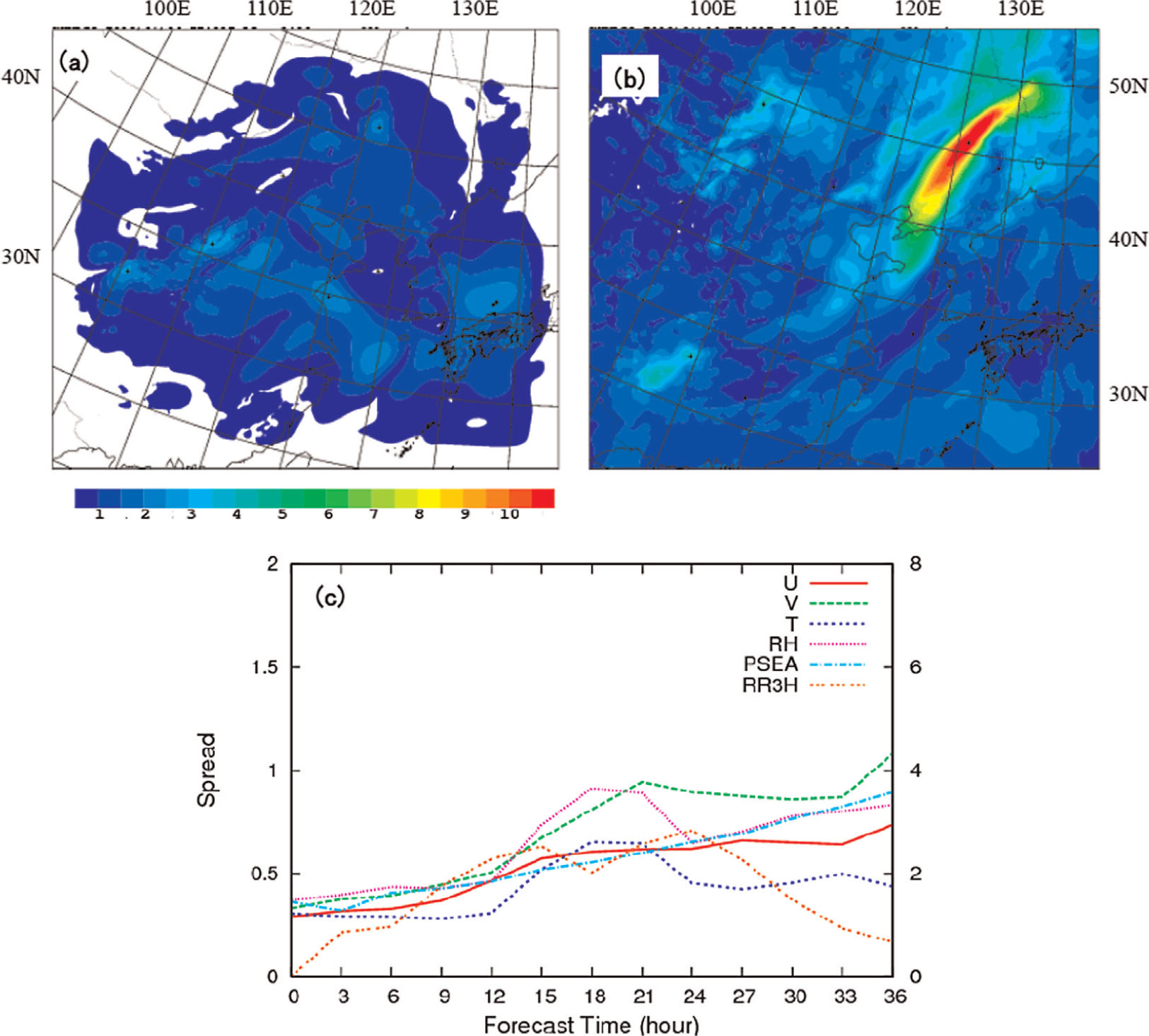
Fig. 8.
Similar to Fig. 7 but with LBPs in both breeding cycles and the ensemble forecast (MBD_lbpfc).
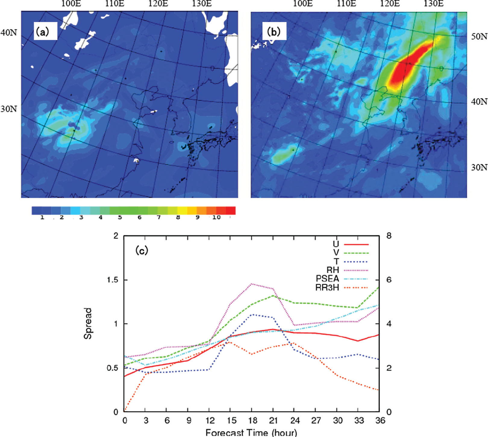
Fig. 9.
Three-hour accumulated precipitation at 12UTC 5 July (FT=24) predicted by each member. From left, member p05, member m05, the ensemble mean and the ensemble spread. (a) MBD method without LBPs (MBD_nlbp). (b) MBD method with LBPs in both breeding cycles and the ensemble forecast (MBD_lbpfc).

Fig. 10.
(a) Averaged RMSEs against initial conditions for 3–4 July 2008 for surface variables. From left to right, Psea, T, RH and V. (b) Same as in (a) but for 500 hPa variables.
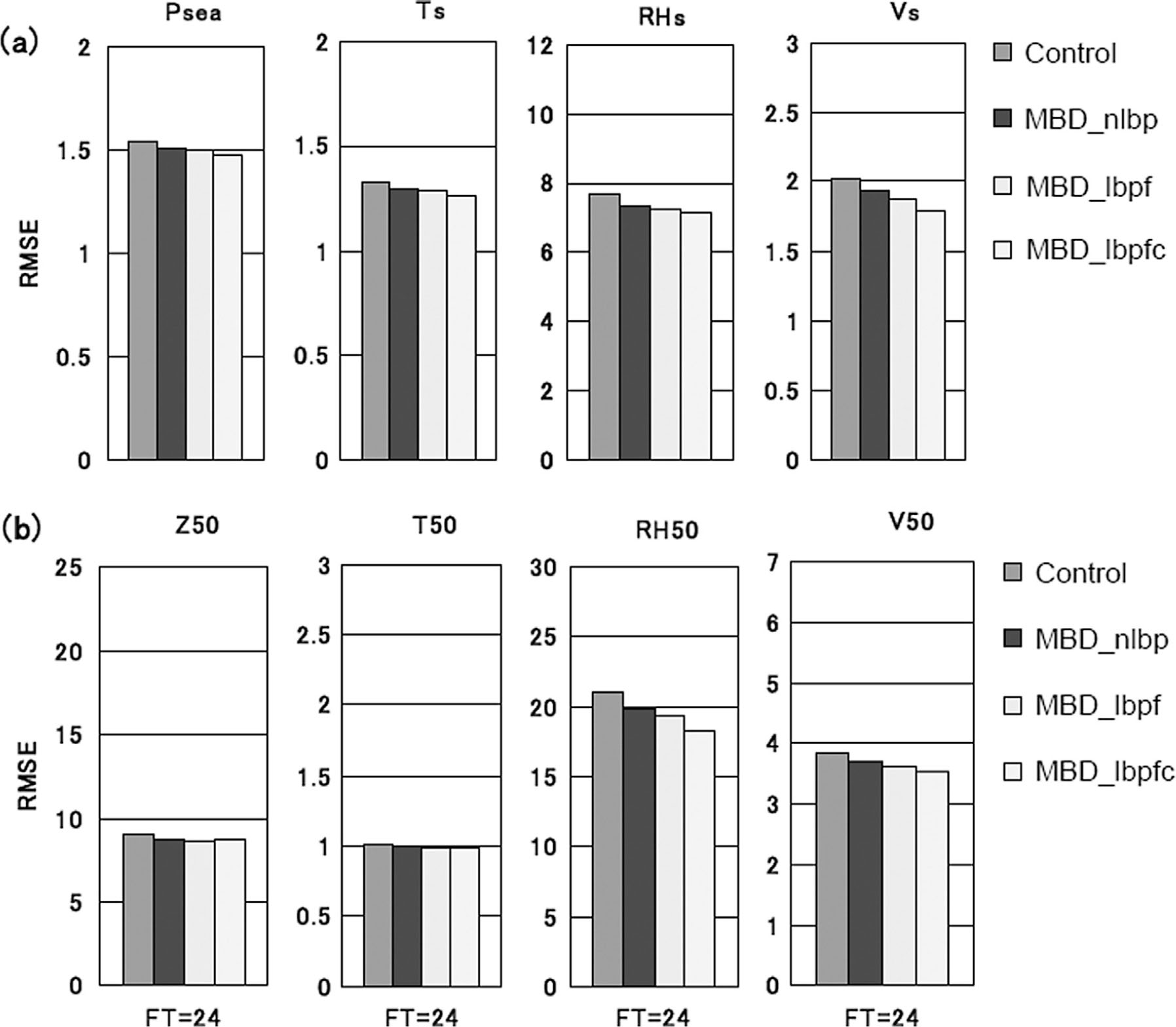
Fig. 11.
Similar to Fig. 7 but for the LET method (LET_lbpf).
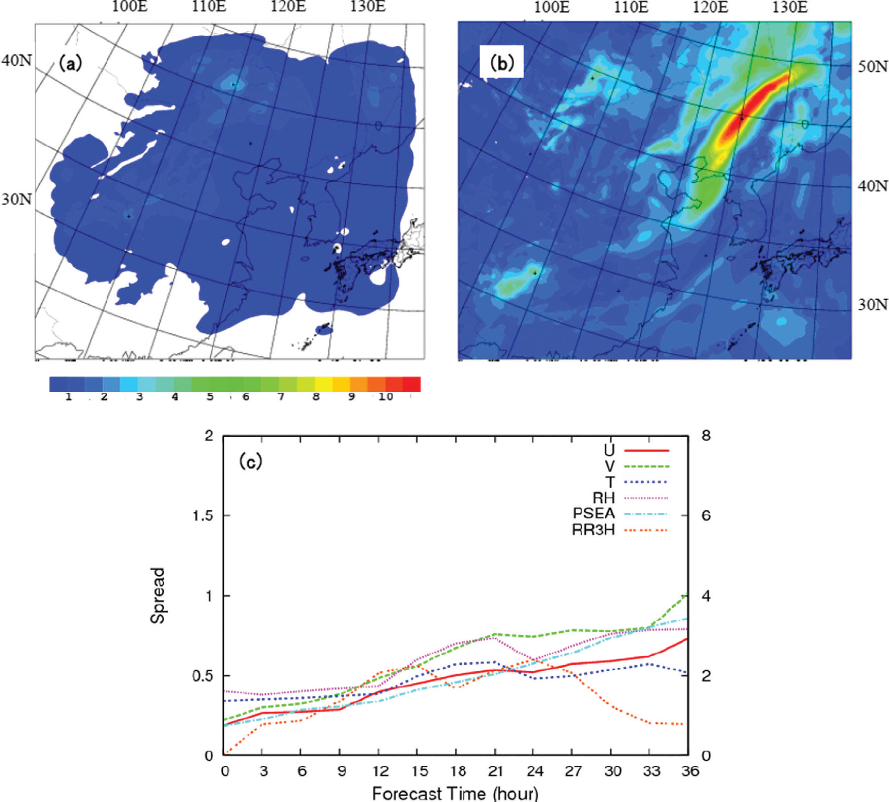
Fig. 12.
Similar to Fig. 11 but with LBPs in both forecast analysis cycles and the ensemble forecast (LET_lbpfc).
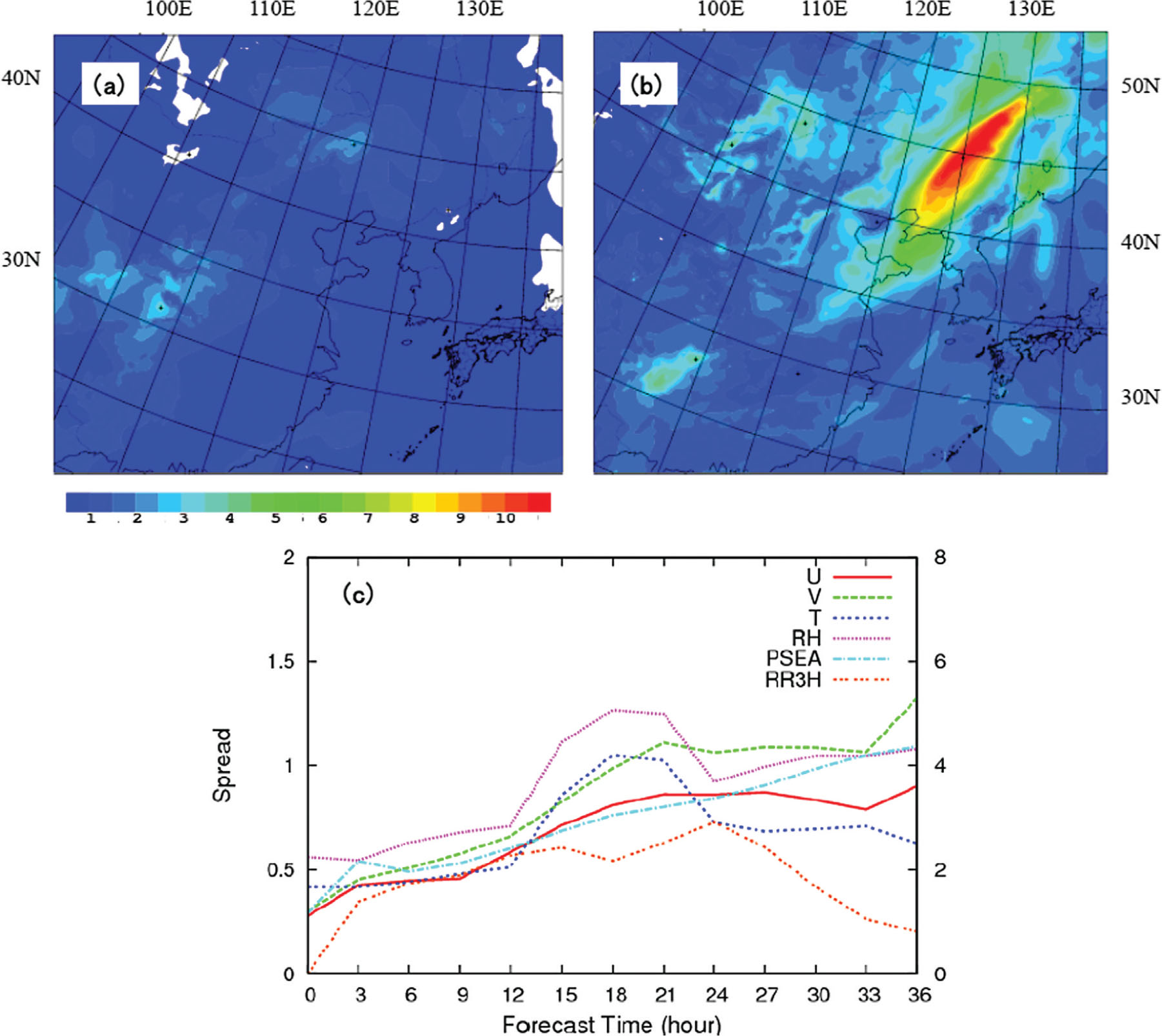
Fig. 13.
Similar to Fig. 10 but for the LET method.
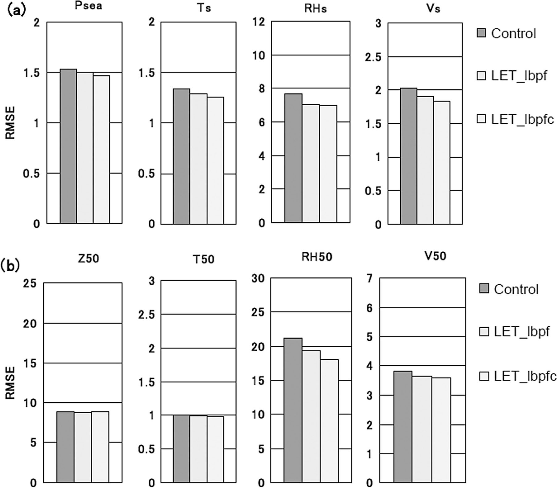
Fig. 14.
(a) Time series of the TE norm. Averages of two EPSs with initial times of 12 UTC, 3 July and 12 UTC, 4 July 2008. (b) Time series of growth rate of TE norm.
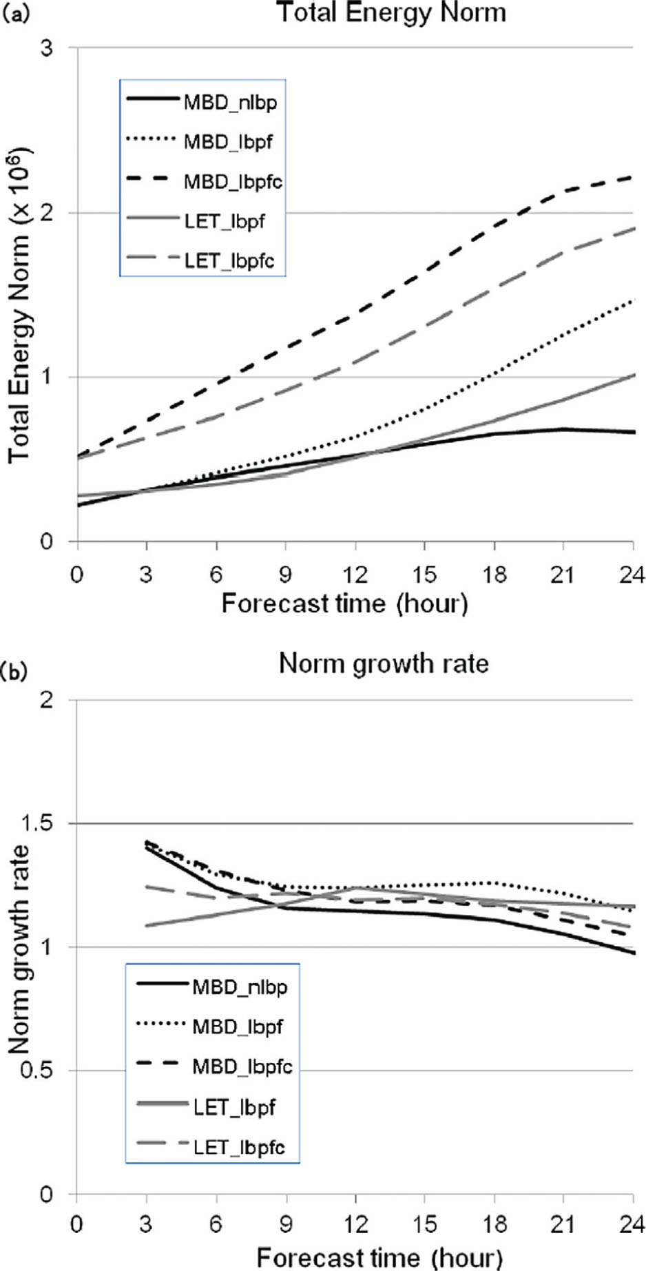
Fig. 15.
Brier Skill Scores against different 6-h precipitation intensity thresholds for the five initial perturbation methods over two 36-h EPSs with initial times of 12 UTC, 3 July, and 12 UTC, 4 July 2008.
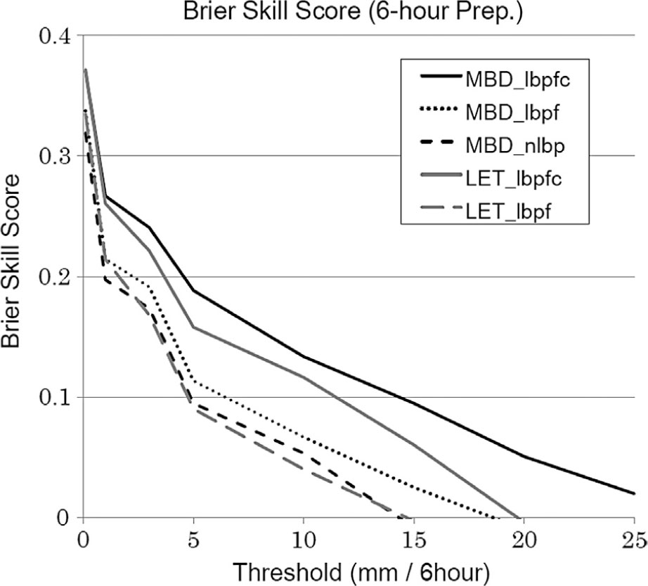
Table 3. (a) Similarity indexes between bred vectors. Upper triangular matrix components indicate the case without LBPs in the breeding cycles (MBD_lbpf), and lower triangular matrix components show the case with LBPs in the breeding cycles (MBD_lbpfc). Values less than −0.4 or greater than 0.4 are indicated in boldface. (b) Same as (a) but for LET initial perturbations. Upper triangular matrix components indicate the case without LBPs in EnKF cycles (LET_lbpf), whereas lower triangular matrix components indicate the case with LBPs in EnKF cycles (LET_lbpfc)
Fig. 16.
Similar to Fig. 4 but by the control run with LETKF analysis (LET_kfbfc).
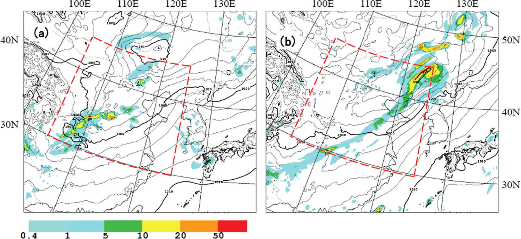
Fig. 17.
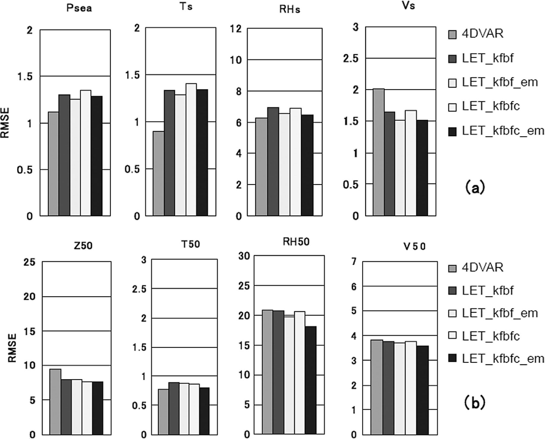
(a) RMSEs of FT=24 forecast fields from 4 July 2008 against the Meso 4D-VAR analysis of 5 July 2008 for surface variables. 4DVAR is the forecast from the 4DVAR analysis, whereas LET_kfbf and LET_kfbfc are forecasts from the LETKF analyses without and with LBPs in EnKF cycles, respectively. LET_kfbf_em and LET_kfbfc_em are their ensemble mean without and with LBPs in EnKF cycles. (b) Same as (a) but for 500 hPa variables.