Fig. 1.
The diabatic cooling as a function of height. Each curve is obtained by eq. (4) with the values of Q s and H Q given by the legend.
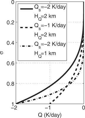
Fig. 2.
The zonally asymmetric 950 h Pa stream function (panels a, c and e) and temperature (b, d and f) responses to prescribed thermal cooling sources that are given in Fig. (1). The thermal cooling is distributed uniformly over the area given by the grey shading but is zero elsewhere. The employed values of Q s and H Q are stated above each panel. The units for the stream funtion and temperature are 106m2s–1 and K, respectively. Negative values are dotted.
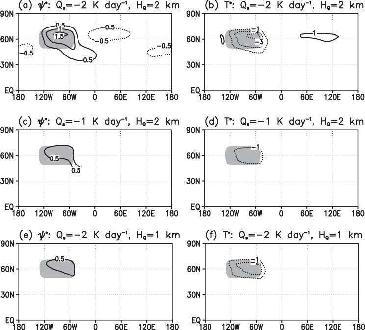
Fig. 3.
The zonally asymmetric stream function response at 950 h Pa to topographic forcing (in 106m2s–1). The topography is given by eq. (15) and its spatial distribution is indicated by the grey shading. However, the topographic forcing is computed differently for each panel: (a) linear topographic response without any thermal cooling, (b) ‘full’ (linear+non-linear) topographic response without any thermal cooling, (c) full topographic response with a surface cooling on the order of Q s =−1Kd–1 and (d) full topographic response with Q s =−2Kd–1. In panels b, c and d, the topographical response was computed with the maximum height of topography set to h 0=2.5km in eq. (15). The linear response in (a) was obtained by running the atmospheric model for 50 model yr (first year discarded as model spin-up) with a lower height of the topography (h 0=250m). The linear stream function anomalies were thereafter multiplied by a factor 10 to account for the lower topography. In the simulations with thermal cooling (panels c and d), the topographical response was obtained by the difference between the response to both topography and thermal cooling (h 0=2.5km, Q s <0) and the response to thermal cooling on a flat surface (h 0=0, Q s <0). The vertical distribution of the thermal forcing is given by eq. (4) using H Q =2km (graphically illustrated in Fig. 1). Horizontally, the thermal forcing is applied uniformly over the topography. Negative values are dotted.
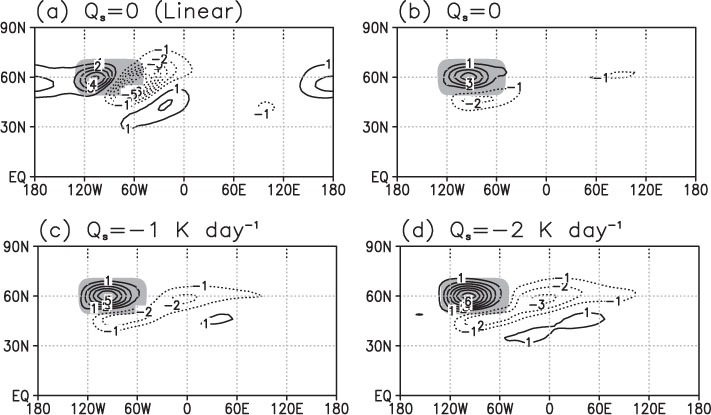
Fig. 4.
Same as Fig. 3 but for the zonally asymmetric temperature (in K) at 950 h Pa.
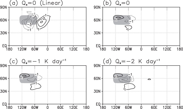
Fig. 5.
Vectors: the difference of the topographically forced perturbation winds (in ms−1) at 950 h Pa between the simulation with both topographical and thermal forcing (h 0=2.5km, Q s <0) and the simulation with topographical forcing in isolation (h 0=2.5km, Q s <0). The topographical response was computed with (a) Q s =−1Kd−1 and (b) Q s =−2Kd−1. Contours: temperature (in K) at 950 h Pa in the simulation with topography and no thermal forcing. The spatial extent of the topography is given by the grey shading.
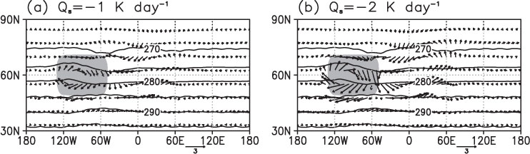
Fig. 6.
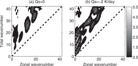
The power spectrum of the topographical forcing in the simulations with idealised topography [eq. (15): h 0=2.5km]. In panel (a) the forcing was obtained by eq. (14) that is conventionally used in linear models. In all other panels, the power spectrum of the full topographical forcing, as given by eq. (8), is shown for the following values of the surface cooling (b) Q s =0, (c) Q s =−1Kd–1and (d) Q s =−2Kd–1. When calculating the power spectrum, the winds at 950 h Pa were used and w was set dimensionless using the planetary radius (6370km) and the rotational frequency of the Earth (7.29×10⁻⁵s–1). The values have been further scaled by 10–15. The dashed line represents the truncation of the model. The topographical forcing is very small for the highest wavenumbers, while only the 30 lowest wavenumbers are shown.
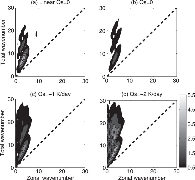
Fig. 7.
The time evolution of the ice sheet in the three ice-sheet simulations conducted in this study. In the control simulation (dashed-dotted line), there are no stationary waves, i.e. T* = 0 in eq. (5) and the climate is zonally uniform. In the ‘Q s =0’ simulation (dashed line), the stationary waves are topographically forced but the thermal cooling induced by the ice sheet is set to zero. In the ‘Q s =−2Kd–1’ simulation (solid line), thermal cooling (given by the solid line in Fig. 1) was added to the topographical forcing. The thermally modified topographical response was computed as follows: First, a simulation was performed both with topography and thermal cooling that were distributed uniformly over the ice-sheet area. Second, another simulation was conducted with the same properties of the thermal cooling field but with no topography (h=0). Finally, the topographically forced response was obtained by taking the difference of the temperature anomalies between the two simulations.
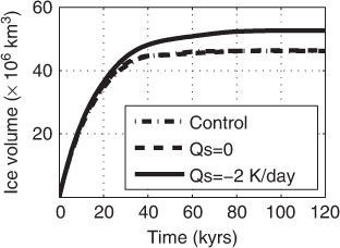
Fig. 8.
The ice thickness (in km; filled contours) and the topographically forced temperature anomalies (in K; coloured contours) at 120kyr in (a) the control, (b) ‘Q s =0’ and (c) ‘Q s =−2Kd–1’ simulations.
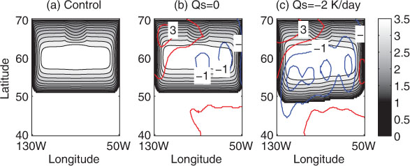
Fig. 9.
Same as in Fig. 3b, d, but with the equilibrium ice-sheet topography (i.e. the ones in Fig. 8b, c) imposed at the lower boundary of the atmospheric model.
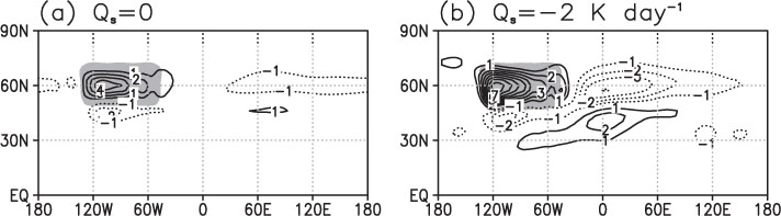
Fig. 10.
Same as Fig. 6b, d, but with the equilibrium ice-sheet topography (i.e. the ones in Fig. 8b, c) was used in the calculation of the topographical forcing. In contrast to Fig. 6, however, the topographical forcing is shown for all the wavenumbers in the atmospheric model.