Fig. 1.
Isotropic energy spectrum and flux in the numerical simulation. Left: energy spectrum, as a function of the wavenumber in units of the inverse of the length of the box, and in units of 1/pixel (between parenthesis). Right: enstrophy flux (solid) and energy flux (dotted), as a function of the wavenumber using the same notation.
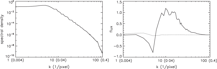
Fig. 2.
Particle and scalar images, DNS and motion estimates. From left to right: Particle (above) and scalar (below) image at time ; Turbulent motion field obtained by DNS in vectorial (above) and colour (below) representation; Motion field inferred by the proposed method and correlation-based velocity fields provided by LaVision in the context of the Fluid FET Open European project (Heitz et al., 2007) for particles (above) and scalar (below). For a better visual analysis, the velocity fields are displayed in a colour representation where colour and intensity code respectively vector orientations and magnitudes (Baker and coauthors, 2007). The corresponding colour map circle is displayed on the left.
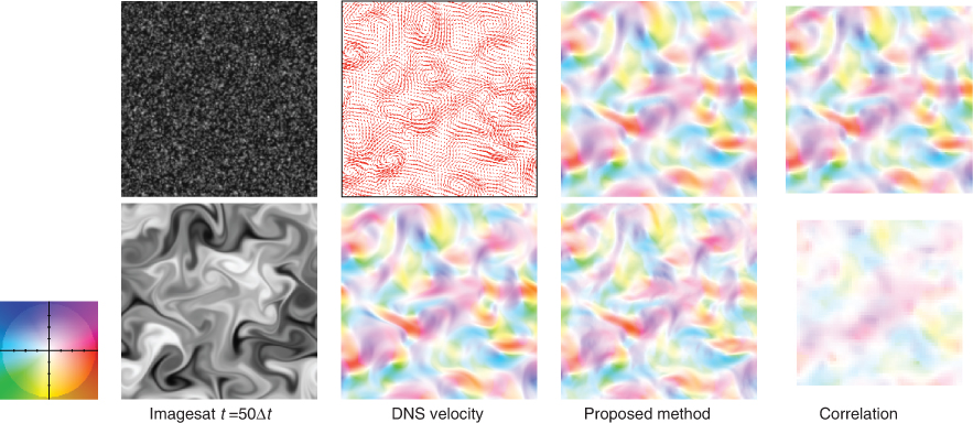
Fig. 3.
Energy of probability and RMS error behaviour w.r.t. power law parameters. Plot of minus of the log of the power law model evidence probability (left) and the motion RMS error (right) w.r.t. power law exponent ζ (ordinate) and prefactor γ (absciss) for the particle (above) and scalar (below) image sequences. The coordinates of the minima are plotted with yellow squares. These coordinates have to be compared with the true power law parameters , given by an LS fit of the DNS data.
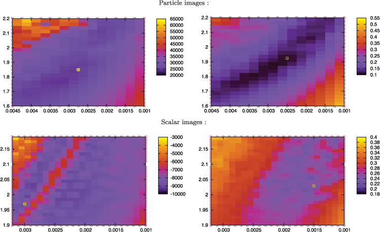
Fig. 4.
Second-order structure function reconstruction. Left plots: Inferred power law model represented by a blue dashed line, and estimated (resp. true) second-order structure function in horizontal-vertical directions plotted with stars (resp. continuous line) and in diagonal directions with cross (resp. dashed line). Right plots: identical legend for the motion estimate obtained with the prior power law model minimising the RMS error.
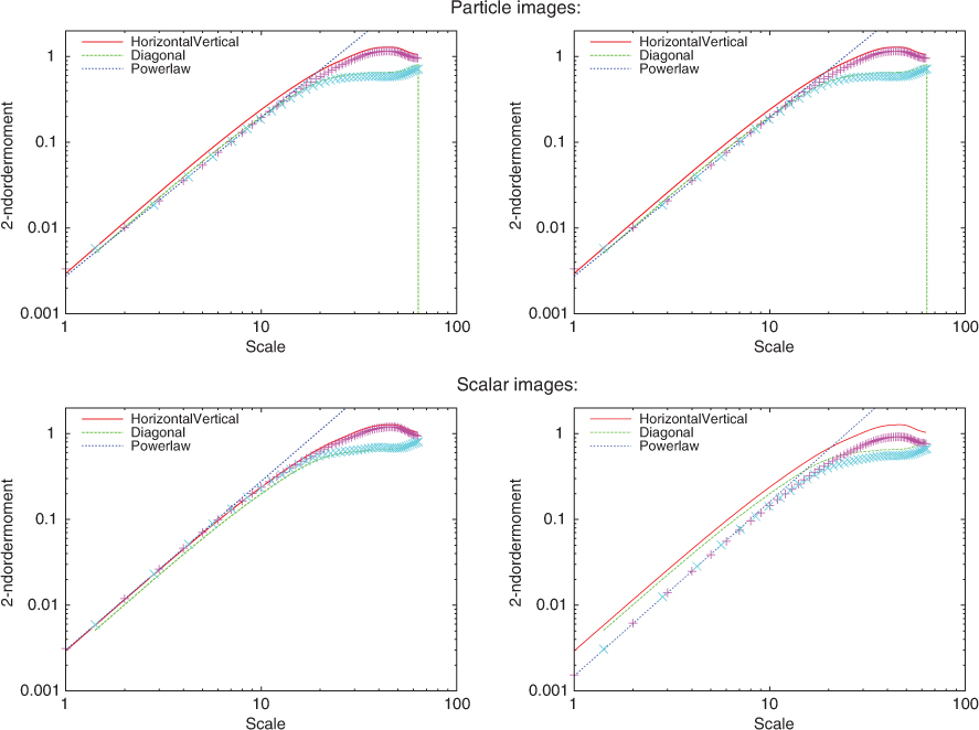
Fig. 5.
Motion estimation accuracy. Evolution of RMS error w.r.t. time index for an operational correlation-based method, a robust first order regularizer (Horn and Schunck, 1981), a second-order regularizer (Yuan et al., 2007), and the inferred self-similar constraints for the particle (left) and scalar (right) image sequences. The results obtained with correlation approach were provided by LaVision (www.lavision.de) company from their operational PIV software (Davis) in the context of the Fluid FET Open European project.
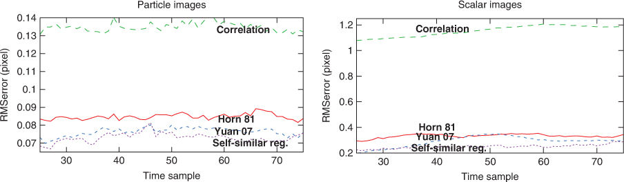
Fig. 6.
Longitudinal structure function exponents and prefactor w.r.t. their order for the scalar image sequence. The proposed self-similar regularization (crosses +) provides exponents (left plots) and prefactors (right plots) (in an LS sense) very close to the ground truth (solid line) in comparison to estimates of (Horn and Schunck, 1981) (stars *) or (Yuan et al., 2007) (× symbols). Correlation-based measurements are not presented here since they do not provide motion increments in the bottom of the scale range of [1, 8] pixels.
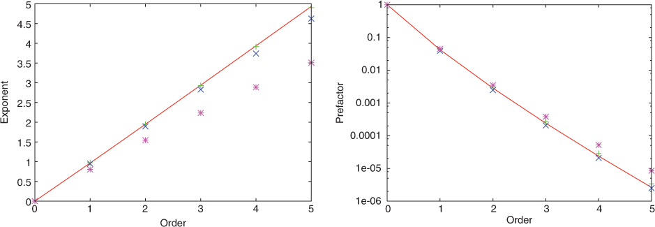
Fig. 7.
Depression over the north-Atlantic Ocean. Sequence of images depicting sparse pressure difference maps of layers at intermediate (above) and low (below) altitude. The images characterise the layers evolution in a time interval of 15 min and with an average spatial resolution of 3 km. Black regions correspond to missing observations and white lines represent meridians (20o, 30o and 40o), parallels (50o and 60o) and the coastal contours of south of Greenland (upper left corner).
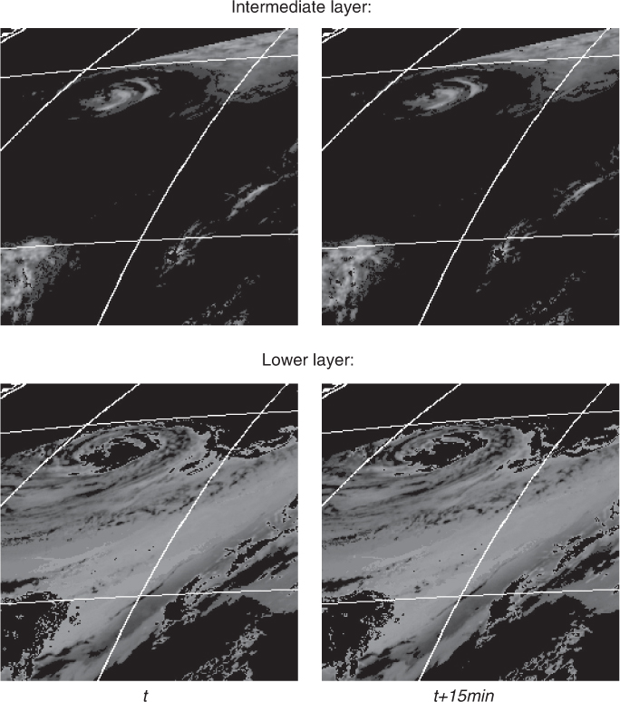
Fig. 8.
Selection of most likely energy flux for Lindborg's model. Minus log of the power law posterior probability vs. energy flux ε in m2 s−3 for horizontal winds at low (solid line) and at intermediate (dashed line) altitude.
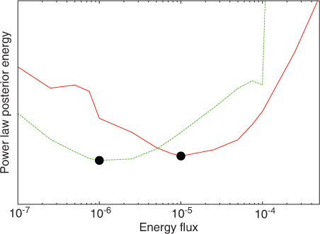
Fig. 9.
Second- (above) and third-(below) order structure functions at low (left column) and intermediate (right column) altitudes. Second-order structure functions (+ symbols) are plotted with their associate models (dashed line). Third-order structure functions (plotted with × symbols for positive values and with + symbols for negative values) can be compared to their associate models (fine dashed line for positive values and coarse dashed line for negative values).
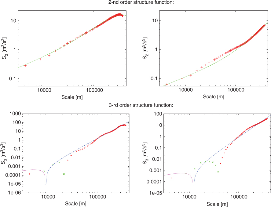
Fig. 10.
Power law evidence probability. Minus log of model probability w.r.t. parameters: exponent ζ (ordinate) and energy flux ɛ in m2 s−3 (absciss) (i.e., prefactor ), for horizontal winds at low (left) and at intermediate (right) altitude. Iso-contours of decreasing values around the minima are plotted in dark blue, yellow and turquoise.
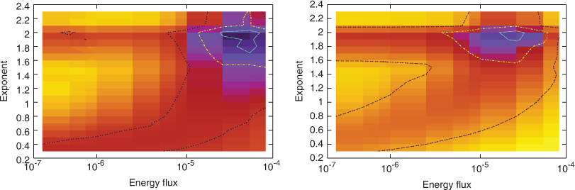
Fig. 11.
Deviation from strict self-similarity at small scales (3–18 km) and at larger scales (30-80 km). Longitudinal structure functions exponents w.r.t. their order at low (solid curve) and intermediate (dashed curve) altitude using the model in (Lindborg and Cho, 2001) (on the left) or a flat prior (on the right) for power law models. The dashed straight lines represent strict self-similar behaviour, i.e., a linear relation of exponents w.r.t. order for the two models.
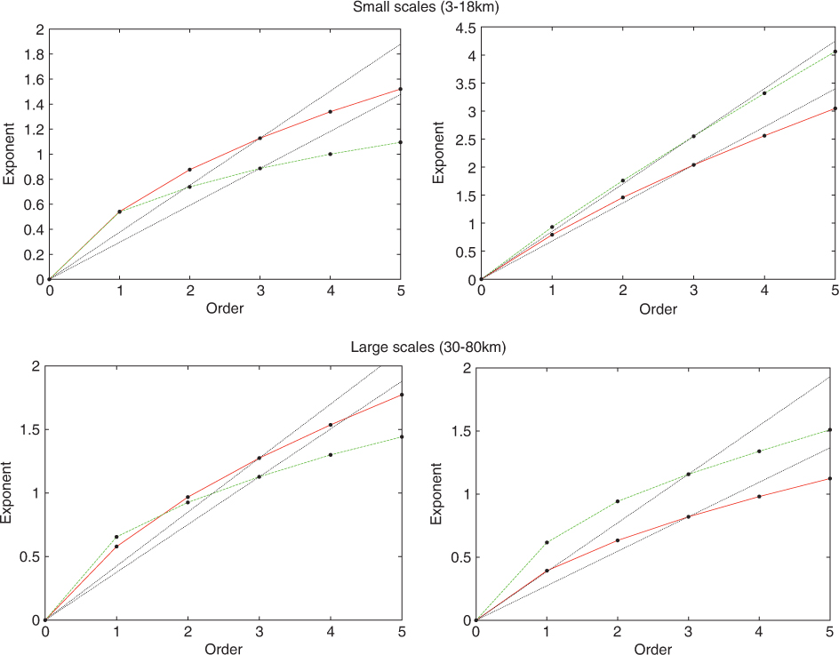
Fig. 12.
Third-order structure functions’ absolute value at low (left) and intermediate (right) altitudes for the two methods. Structure functions obtained with a (Lindborg and Cho, 2001) (resp. a flat) prior are plotted with×symbols (resp. □symbols) for positive values and with + symbols (resp. * symbols) for negative values. Estimate obtained with the (Lindborg and Cho, 2001) prior can be compared to their associate models (fine dashed curve for positive values and coarse dashed curve for negative values). At large scales, estimate obtained with both priors scale as ∼ℓ3 (straight dashed line).
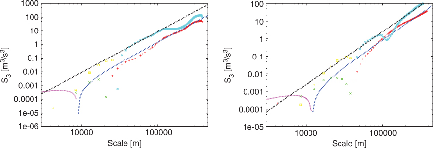
Fig. 13.
Estimated horizontal wind fields compared to correlation results. Dense wind fields at low (left) and intermediate (right) altitude where obtained using the flat prior, i.e., a scaling in ℓ2. The correlation results were obtained using the operational PIV software (Davis) from LaVision (http:\\www.lavision.de) company.
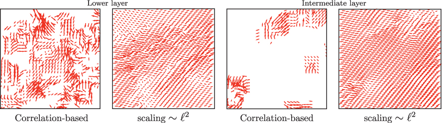
Fig. 14.
Detail of horizontal winds at low altitude. From top to bottom: input image (zoom between the 20o and 30o meridians and the 50o and 60o parallels), solenoidal (2 following lines) and divergent part (2 last lines) of motion estimated with a scaling of ℓ2/3 (second and fourth line) or ℓ2 (third and fifth line).
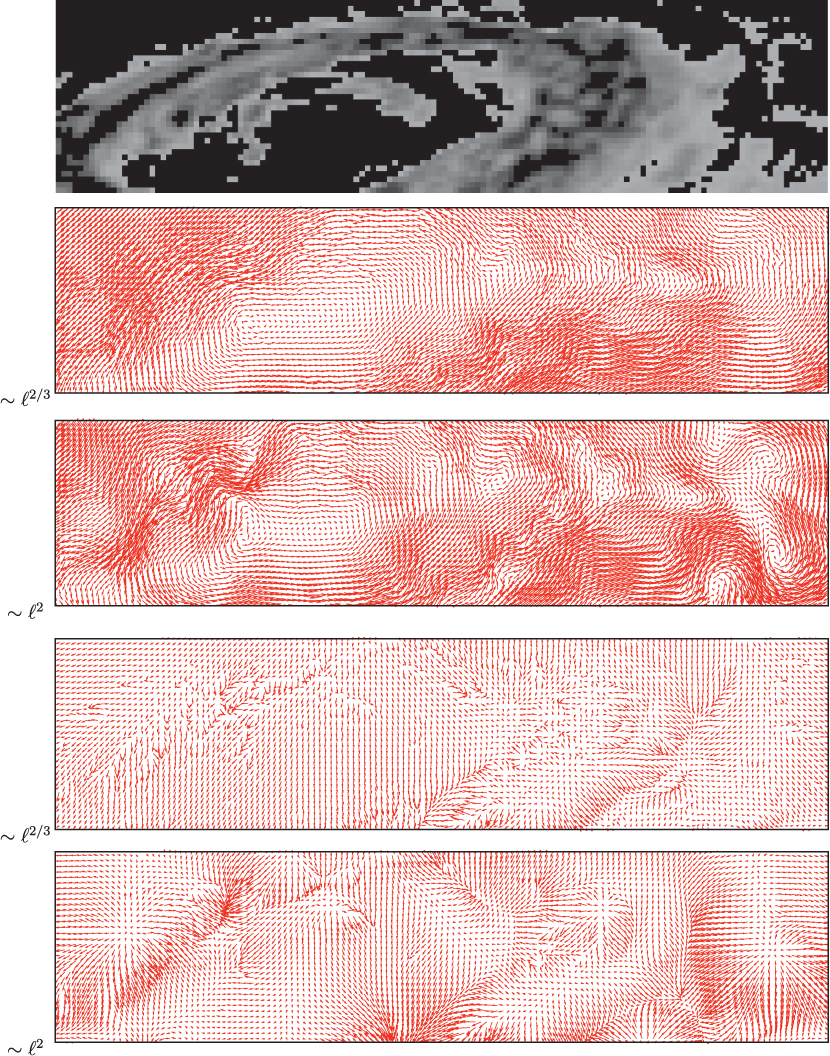
Fig. 15.
Detail of horizontal winds at intermediate altitude. From top to bottom: input image (zoom between the 20o and 30o meridians and the 50o and 60o parallels), solenoidal (2 following lines) and divergent part (2 last lines) of motion estimated with a scaling of ℓ2/3 (second and fourth line) or ℓ2 (third and fifth line).
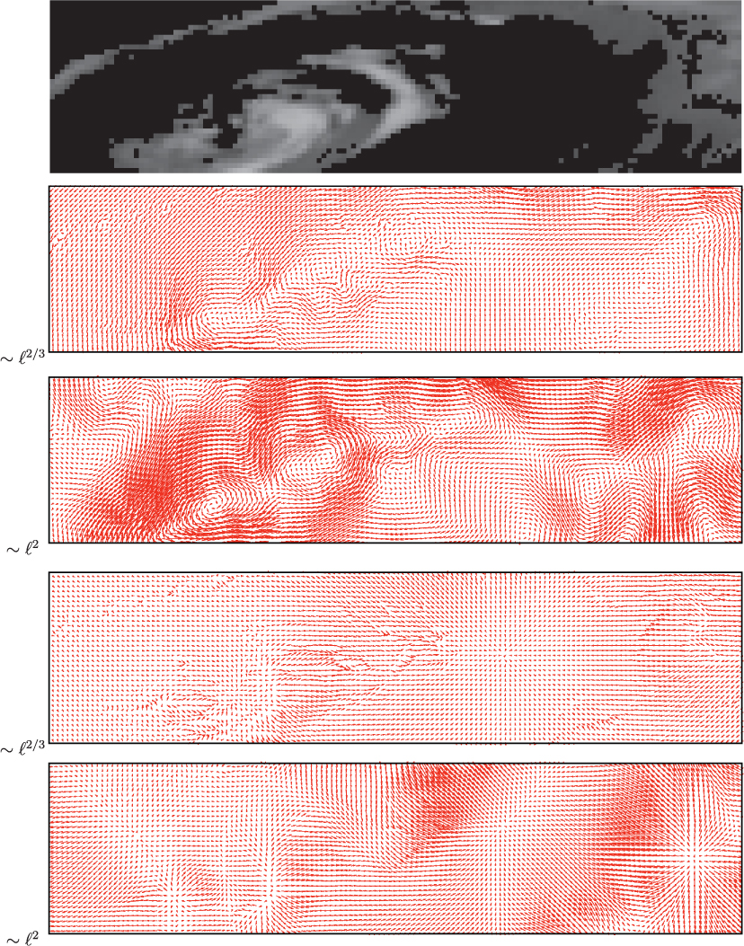
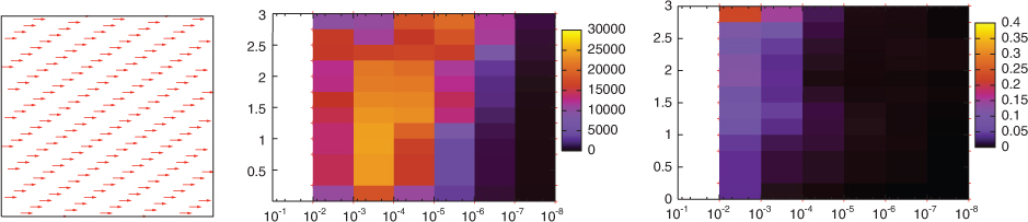
Fig. 16.
Power law evidence probability for laminar flows. True velocity field (left), plot of minus of the log of the power law model probability (centre) and the RMS motion reconstruction error (right) w.r.t. power law exponent ζ (ordinate) and prefactor γ (absciss). The line of minima which is selected by Bayesian inference corresponds to the true underlying power law (γ=0 for any ζ).