
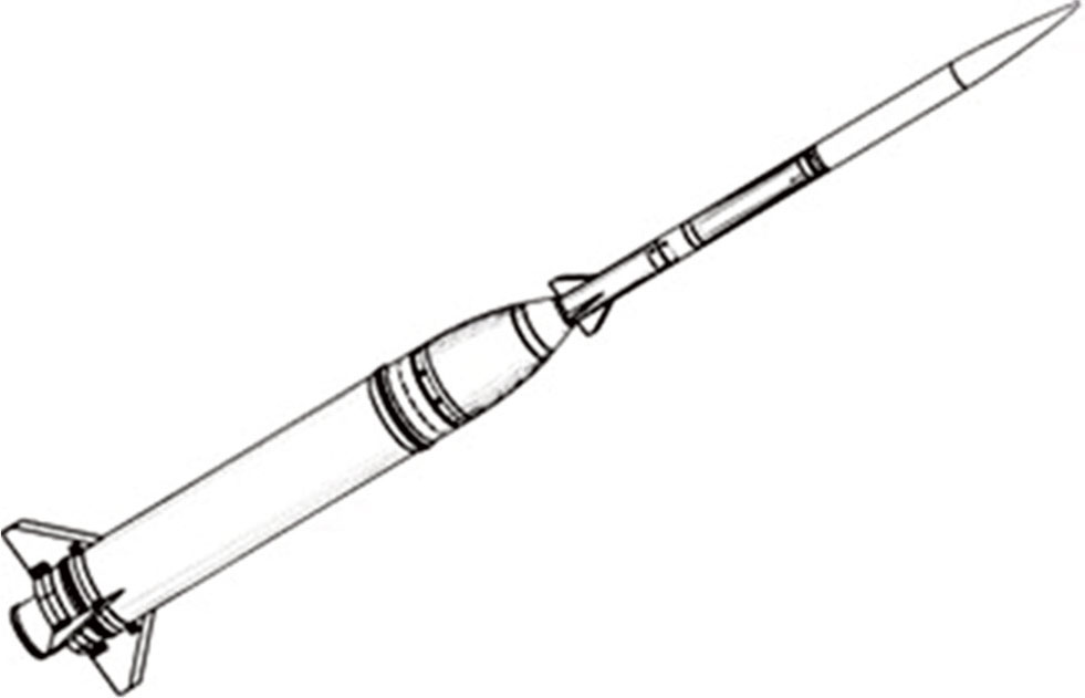
Figure 1.
Visualisation of the Grot sounding rocket.
Table 1.
Grot main dimensional parameters.
| Parameter | Value [m] |
|---|---|
| Total rocket length | 2.000 |
| First stage length | 0.983 |
| Second stage length | 1.017 |
| First stage diameter | 0.135 |
| Second stage diameter | 0.045 |
| Reference diameter | 0.135 |
| Pre-flight distance of centre of mass from the rocket’s base | 0.979 |
| Nozzle exit diameter | 0.084 |
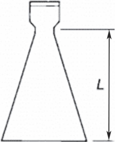
Figure 2.
Conical rocket nozzle [7].
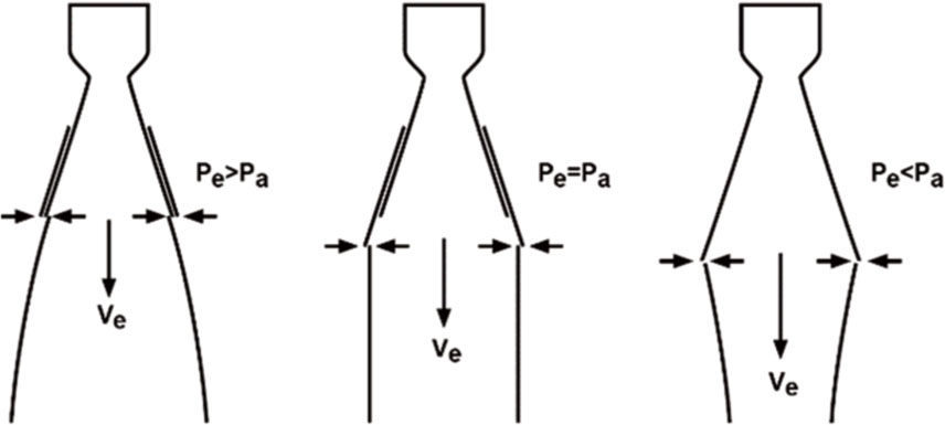
Figure 3.
From left to right: (A) under-expanded nozzle, (B) ideally expanded nozzle and (C) over-expanded nozzle; based on http://www.braeunig.us/space/sup1.htm.

Figure 4.
Axial forces acting on the Grot rocket.
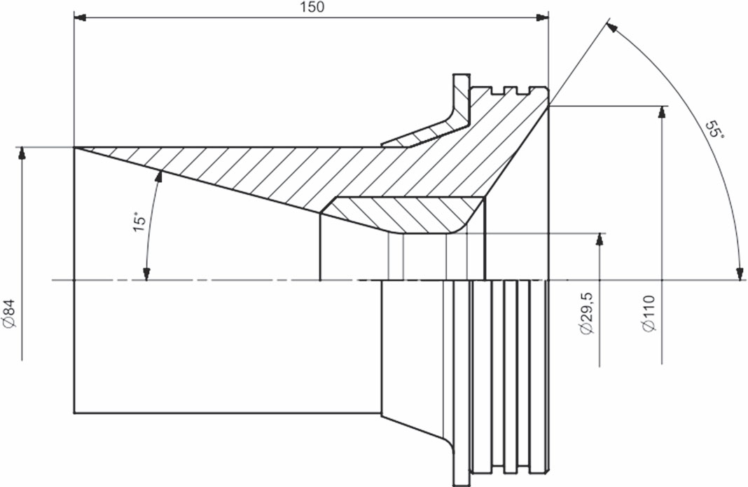
Figure 5.
Technical drawing of Grot’s nozzle.

Figure 6.
Grot’s shape outlines and domain regions in Ansys® DesignModeler.
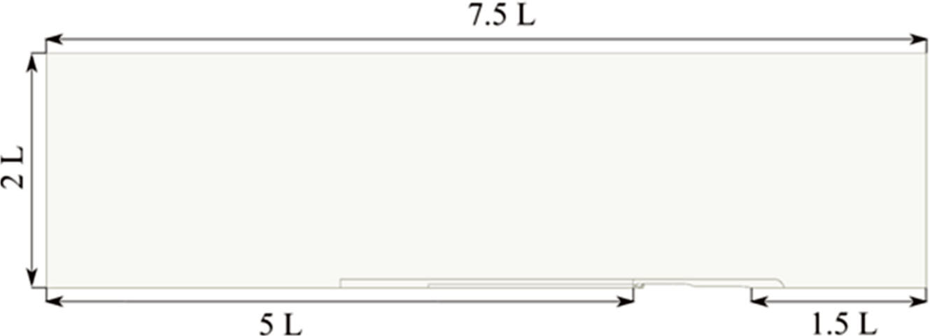
Figure 7.
Fluid domain dimensions. L denotes the total length of the Grot sounding rocket.
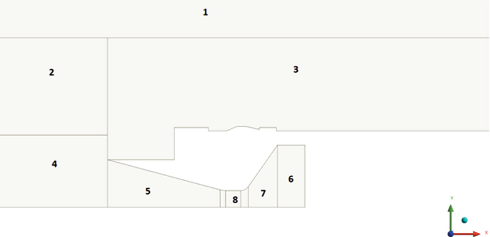
Figure 8.
Fluid domain regions.
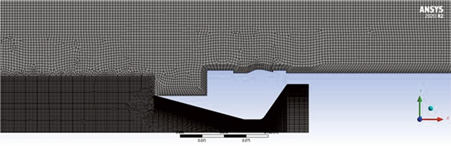
Figure 9.
Near-nozzle mesh.
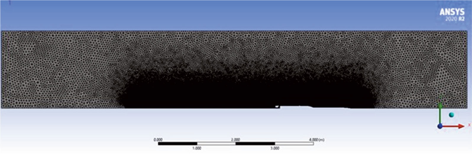
Figure 10.
Global view of the mesh.
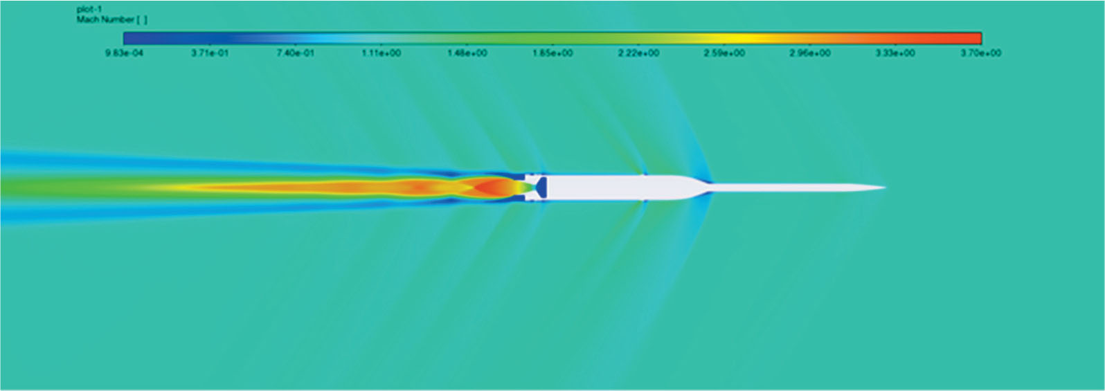
Figure 11.
Contour plot of the local Mach number—active propulsion system, Mach 1.2.
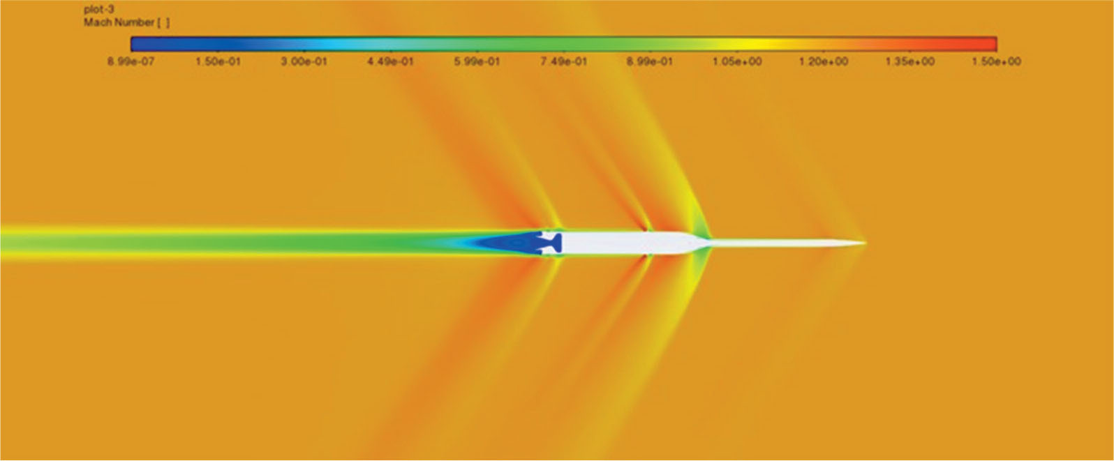
Figure 12.
Contour plot of the local Mach number— inactive propulsion system, Mach 1.2.
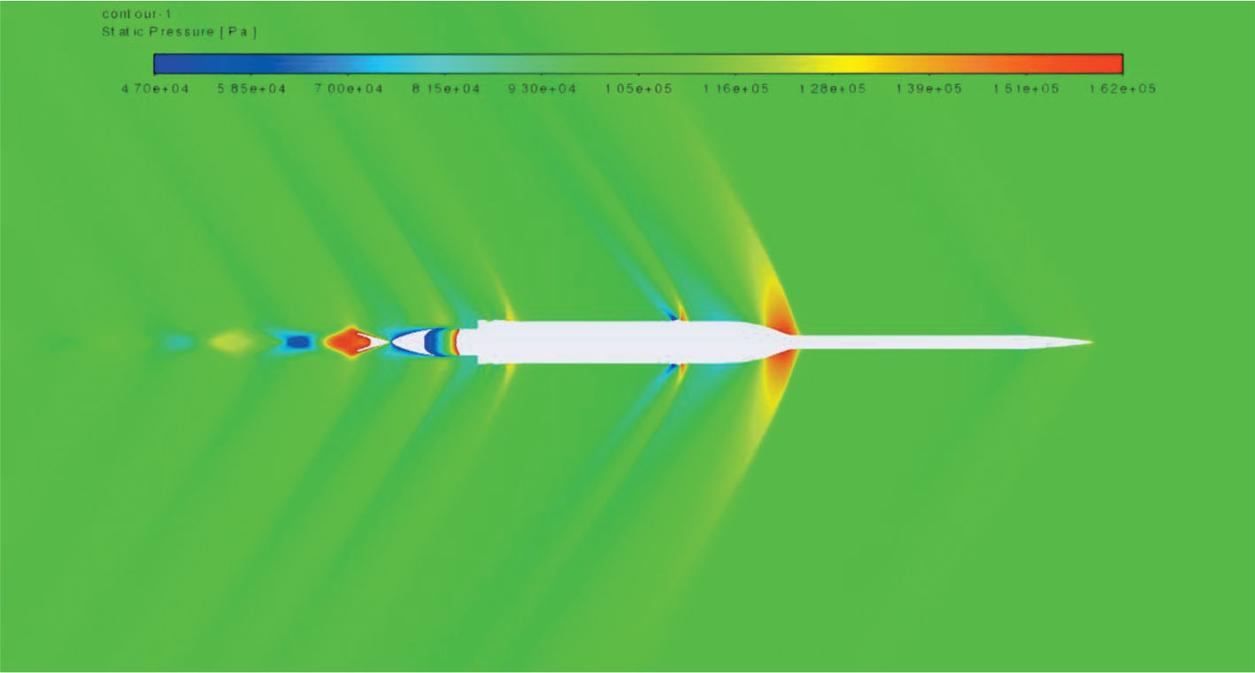
Figure 13.
Contour plot of the local static pressure—active propulsion system, Mach 1.2.
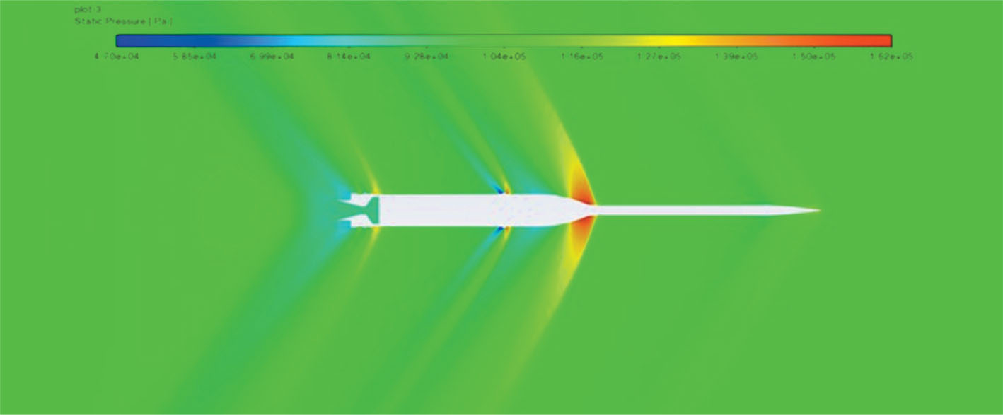
Figure 14.
Contour plot of the local static pressure—inactive propulsion system, Mach 1.2.
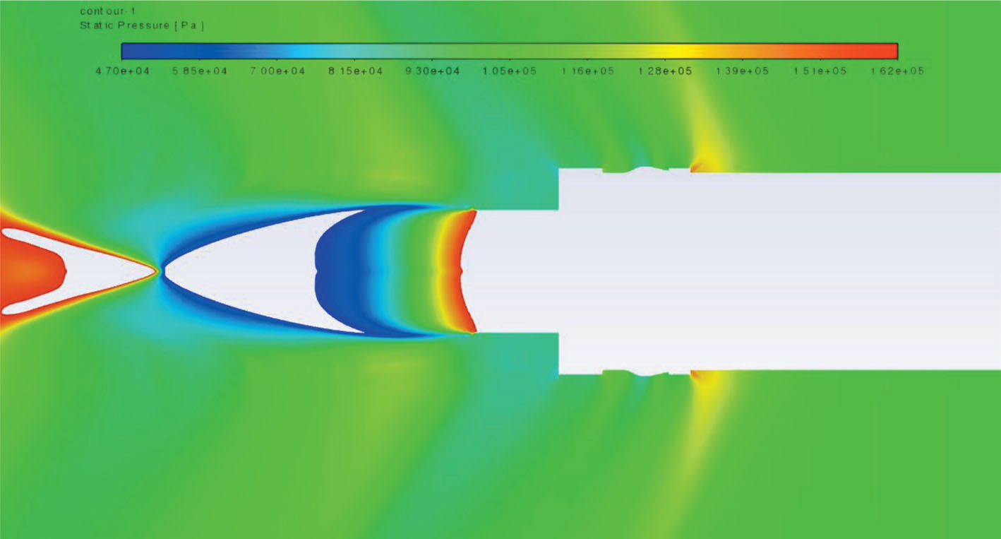
Figure 15.
Contour plot of the local static pressure in the nozzle area—active propulsion system, Mach 1.2.
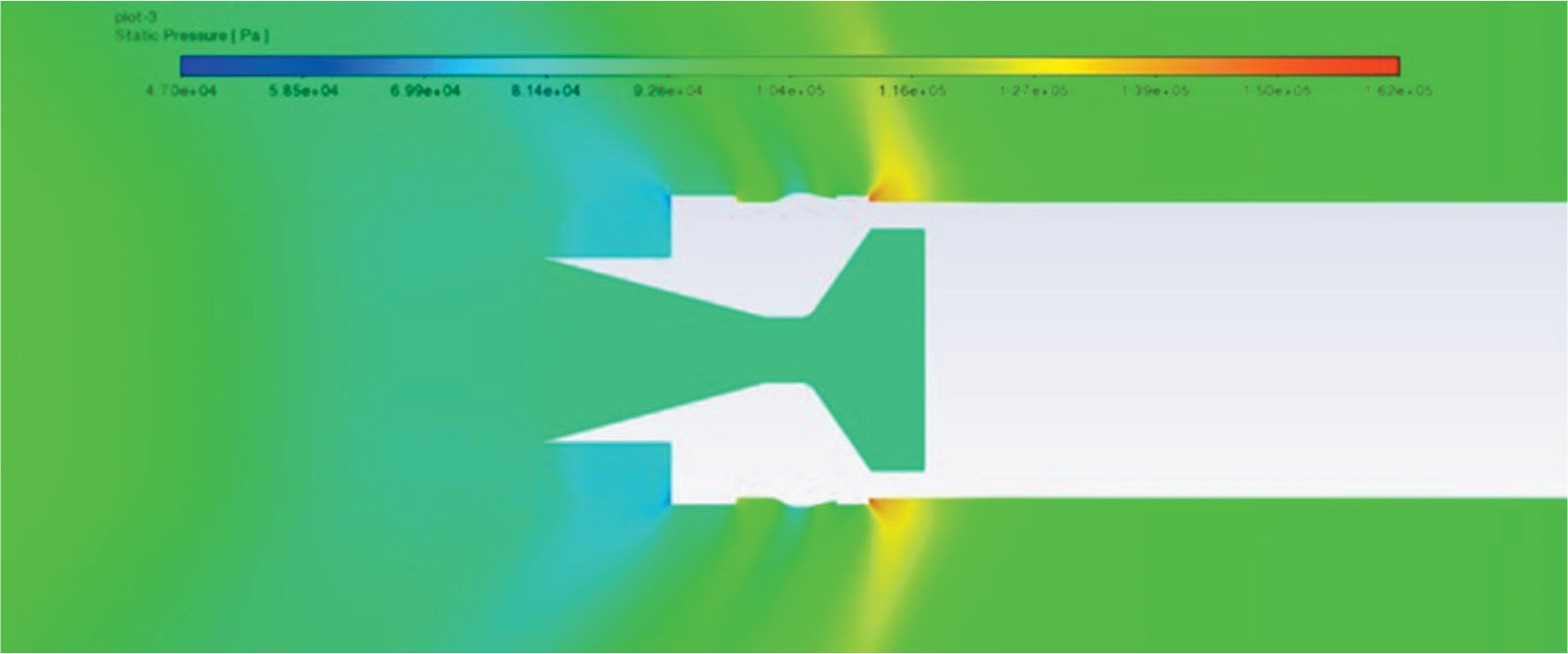
Figure 16.
Contour plot of the local static pressure in the nozzle area—inactive propulsion system, Mach 1.2.
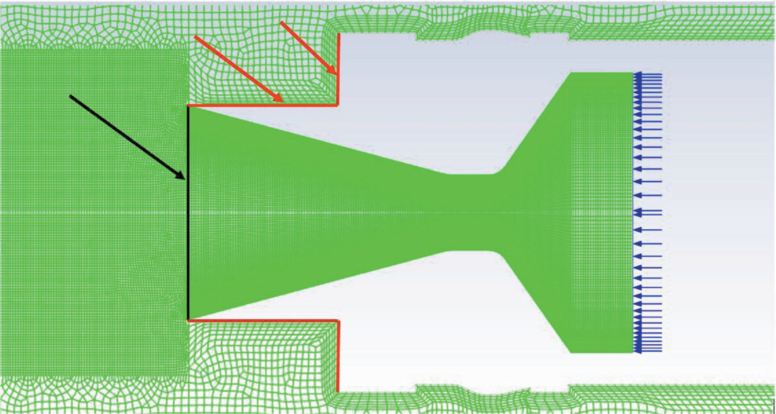
Figure 17.
Areas of interest in the rear of the rocket. Black denotes the nozzle exit area, while red denotes the aft end.
Table 2.
Computed drag coefficients.
| M [-] | ΔCD[–] | ||
|---|---|---|---|
| 0.3 | 0.460 | 0.453 | -0.007 |
| 0.6 | 0.378 | 0.457 | 0.079 |
| 0.8 | 0.359 | 0.462 | 0.100 |
| 1.0 | 0.494 | 0.668 | 0.170 |
| 1.2 | 0.628 | 0.744 | 0.120 |
| 1.6 | 0.577 | 0.659 | 0.080 |
| 2.0 | 0.506 | 0.576 | 0.070 |
| 2.5 | 0.435 | 0.495 | 0.060 |
| 3.0 | 0.383 | 0.429 | 0.046 |
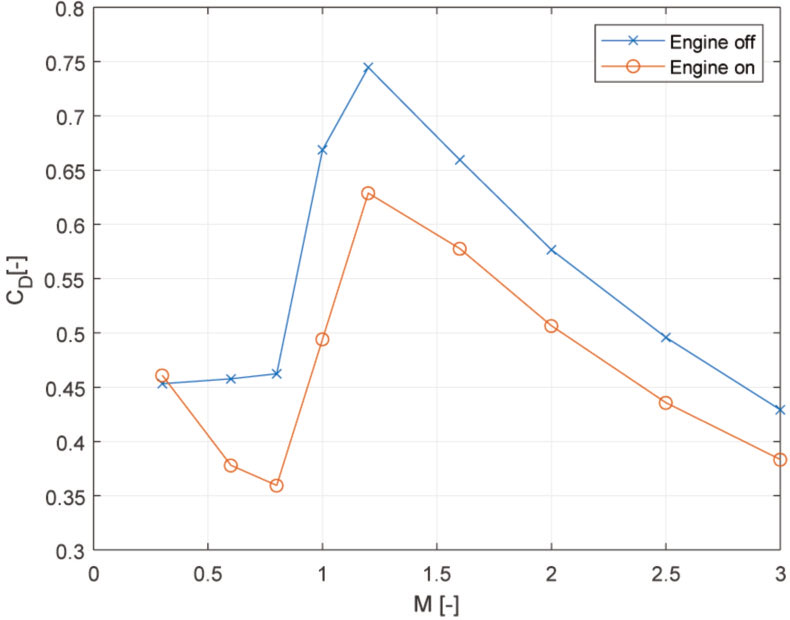
Figure 18.
Total drag coefficient as a function of Mach number.
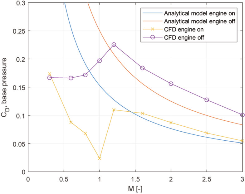
Figure 19.
Comparison of base drag coefficients obtained by CFD and the analytical model found in [4].
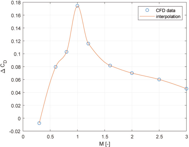
Figure 20.
Difference in the total drag coefficient between active and inactive propulsion systems. Interpolation performed by the modified Akima method.
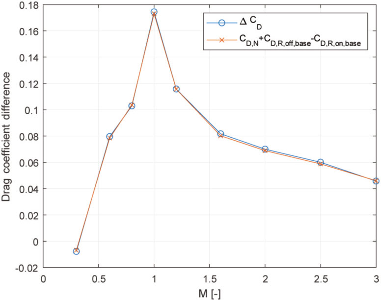
Figure 21.
ΔCD compared to the sum of engine-off nozzle exit pressure drag Coff and pressure change in the aft end due to engine operation.
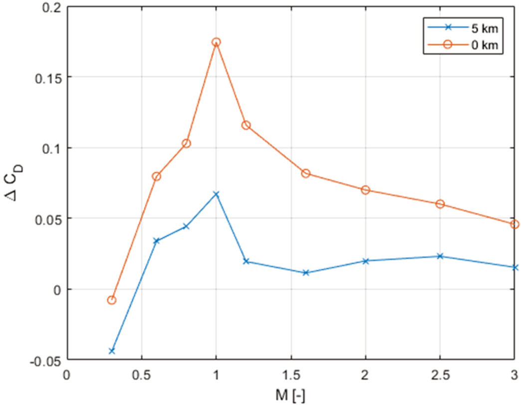
Figure 22.
ΔCD for altitudes of 0 km and 5 km.