
Table 1:
Sieve size with different percentages of fines.
| Sieve size | Gradation with 3% fines | Gradation with 6% fines | Gradation with 9% fines | |||
|---|---|---|---|---|---|---|
| % Passing | % Retained | % Passing | % Retained | % Passing | % Retained | |
| 3/4″ | 100 | 0 | 100 | 0 | 100 | 0 |
| 1/2″ | 80 | 20 | 85 | 15 | 86 | 14 |
| 3/8″ | 67 | 13 | 70 | 13 | 74 | 12 |
| #4 | 47 | 20 | 57 | 20 | 54 | 20 |
| #8 | 28 | 19 | 37 | 20 | 34 | 20 |
| #16 | 9 | 19 | 17 | 20 | 14 | 20 |
| #200 | 4 | 5 | 12 | 5 | 9 | 5 |
| Pan | 3 | 6 | 9 | |||
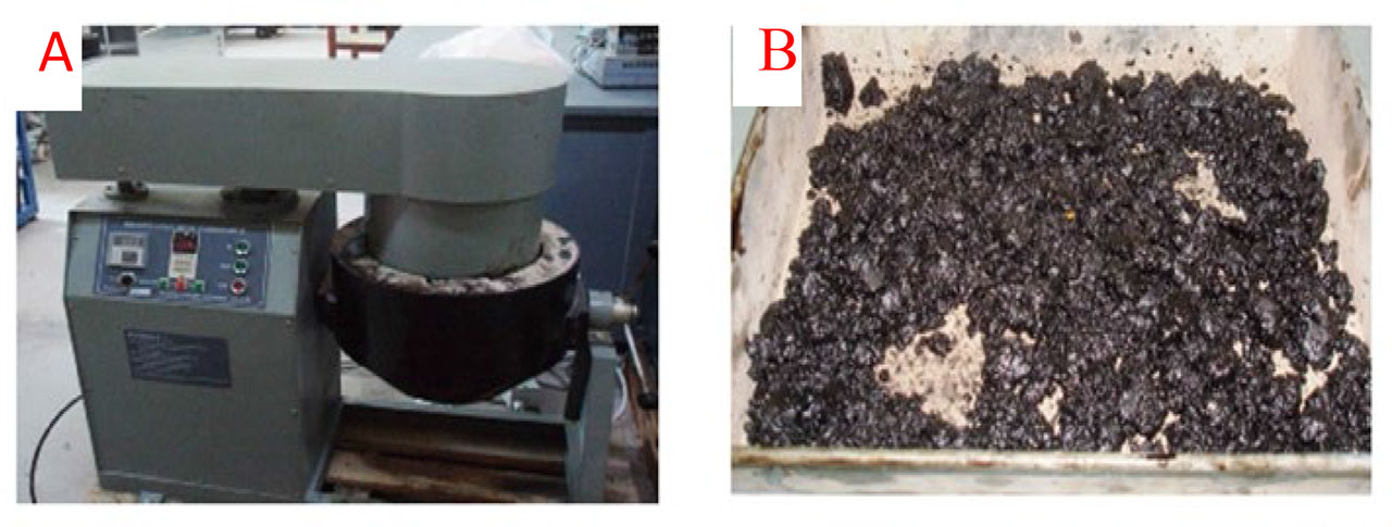
Figure 1:
A) Mixing of aggregates and bitumen in a mechanical mixing machine, B) loose mixture prepared for conditioning.
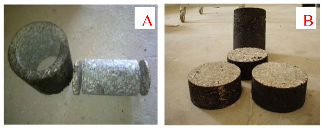
Figure 2:
A) Core and trimmed specimen along with waste rings for SPT; B) core specimens for IDT.
Table 2:
Peak load values in indirect tensile strength test.
| Fines | Controlled unconditioned | Controlled conditioned | Antistripped and conditioned |
|---|---|---|---|
| 3% | 9200 (N) | 7200 (N) | 8000 (N) |
| 6% | 9500 (N) | 7600 (N) | 8500 (N) |
| 9% | 9100 (N) | 7000 (N) | 7700 (N) |
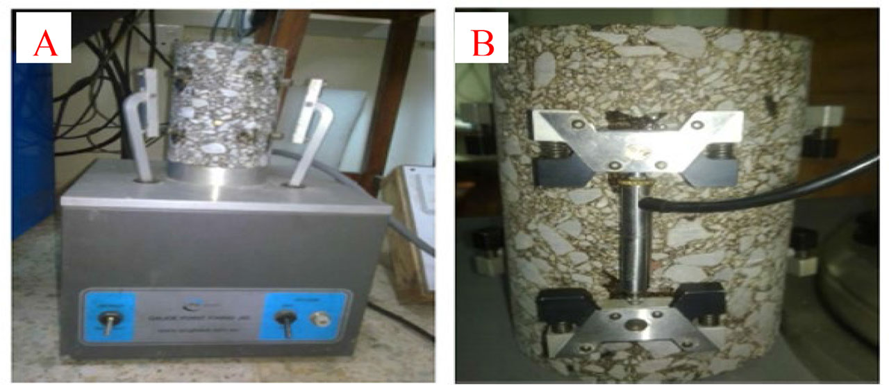
Figure 3:
A) Studs fixing using gauge point fixing device; B) clamps and LVDTs mounted on the sample.
Table 3:
Job mix formula observations for mix having 3%, 6%, and 9% fines (ASTM Standard, D-3515, 2014).
| Parameters | Criteria | Measured Value | Remarks (3%/6%/9%) | ||
|---|---|---|---|---|---|
| 3% fines | 6% fines | 9% fines | |||
| Optimum asphalt content (%) | NA | 4.10 | 4.45 | 5.00 | P/P/P |
| VMA (%) | 14 | 14.10 | 14.10 | 16.60 | P/P/P |
| VFA (%) | 65–75 | 71.00 | 71.00 | 71.00 | P/P/P |
| Stability (N) | 8006 | 8630 | 8465 | 8110 | P/P/P |
| Flow (mm) | 2.0–3.5 | 2.55 | 2.85 | 3.10 | P/P/P |
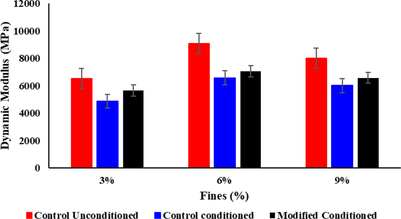
Figure 4:
Measured dynamic modulus of asphalt concrete mixtures with 3%, 6%, and 9% fines with and without freeze–thaw conditioning.
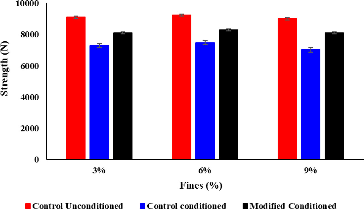
Figure 5:
IDT strength of asphalt concrete mixtures with 3%, 6%, and 9% fines with and without freeze–thaw conditioning.
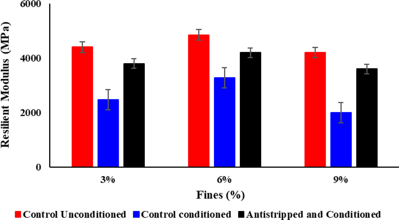
Figure 6:
Measured resilient modulus of asphalt concrete mixtures with 3%, 6%, and 9% fines with and without freeze–thaw conditioning.
Table 4:
Comparison of different parameters for moisture susceptibility.
| Fines (%) | Conditioning | Dynamic modulus ratio at 10 (Hz) | Tensile strength ratio | Resilient modulus ratio | |||
|---|---|---|---|---|---|---|---|
| Without AS | With AS | Without AS | With AS | Without AS | With AS | ||
| 3% | One cycle F-T | 74 | 85 | 78 | 87 | 56 | 87 |
| 6% | One cycle F-T | 74 | 81 | 80 | 89 | 68 | 90 |
| 9% | One cycle F-T | 69 | 80 | 77 | 85 | 51 | 86 |
Table 5:
Factor's notations and their levels for analysis.
| Factors | Notation | Levels | |
|---|---|---|---|
| Frequency (Hz) | A | 0.1 | 25 |
| Fines (%) | B | 3 | 9 |
| Conditioning | C | Conditioned | Unconditioned |
Table 6:
Measured values of dynamic modulus with different percent fines and frequency.
| Frequency (Hz) | Fines (%) | Conditioning | Dynamic modulus (MPa) |
|---|---|---|---|
| 0.1 | 3 | Conditioned | 805 |
| 0.1 | 3 | Conditioned | 1036 |
| 0.1 | 9 | Conditioned | 1100 |
| 25 | 3 | Conditioned | 5704 |
| 25 | 3 | Unconditioned | 7474 |
| 25 | 3 | Conditioned | 6268 |
| 25 | 9 | Conditioned | 7501 |
| 0.1 | 9 | Conditioned | 845 |
| 25 | 9 | Unconditioned | 10.376 |
| 25 | 9 | Conditioned | 7091 |
| 0.1 | 3 | Unconditioned | 963 |
| 0.1 | 9 | Unconditioned | 1423 |
| 25 | 9 | Unconditioned | 10.508 |
| 25 | 3 | Unconditioned | 7124 |
| 0.1 | 3 | Unconditioned | 966 |
| 0.1 | 9 | Unconditioned | 1550 |
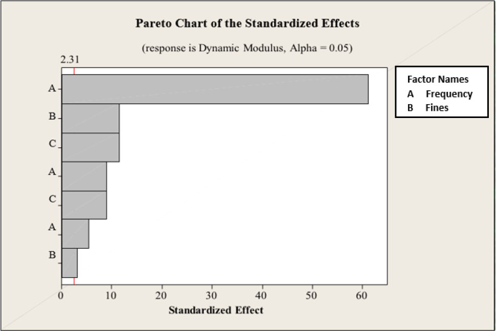
Figure 7:
Pareto plot illustrating standardized effects.
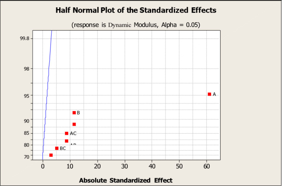
Figure 8:
Visualization of absolute standardized effects in the half-normal plot.
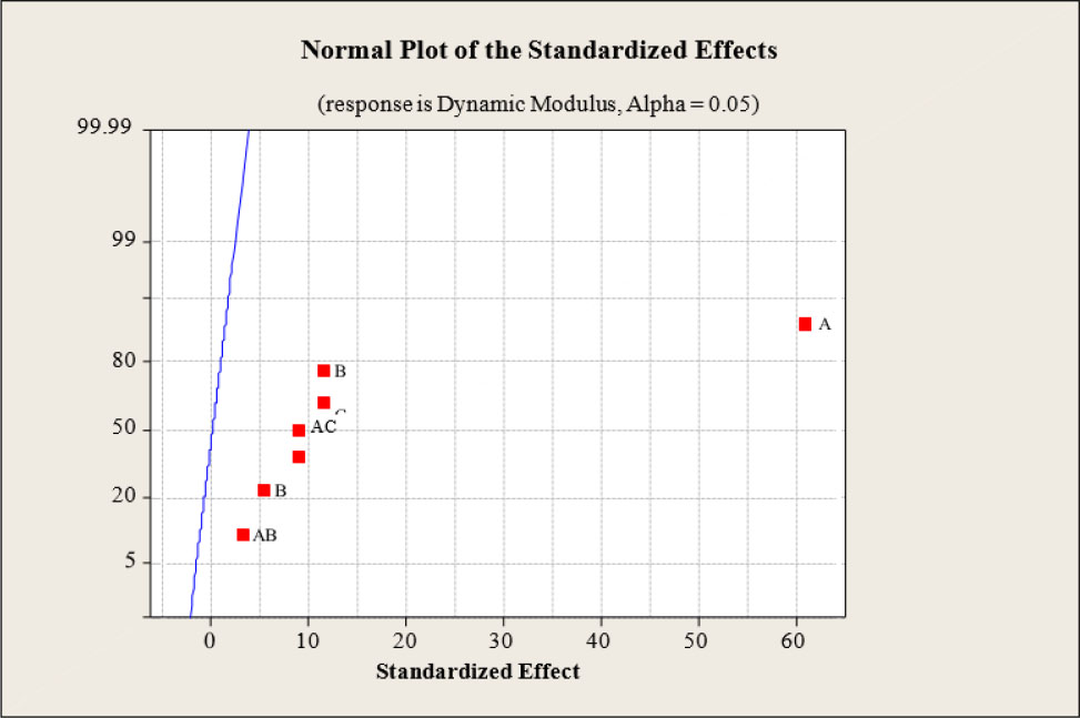
Figure 9:
Visualization of the standardized effect of the normal plot.
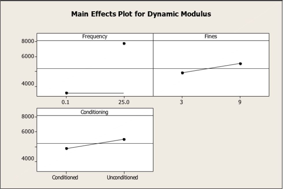
Figure 10:
Main effects plot for dynamic modulus.
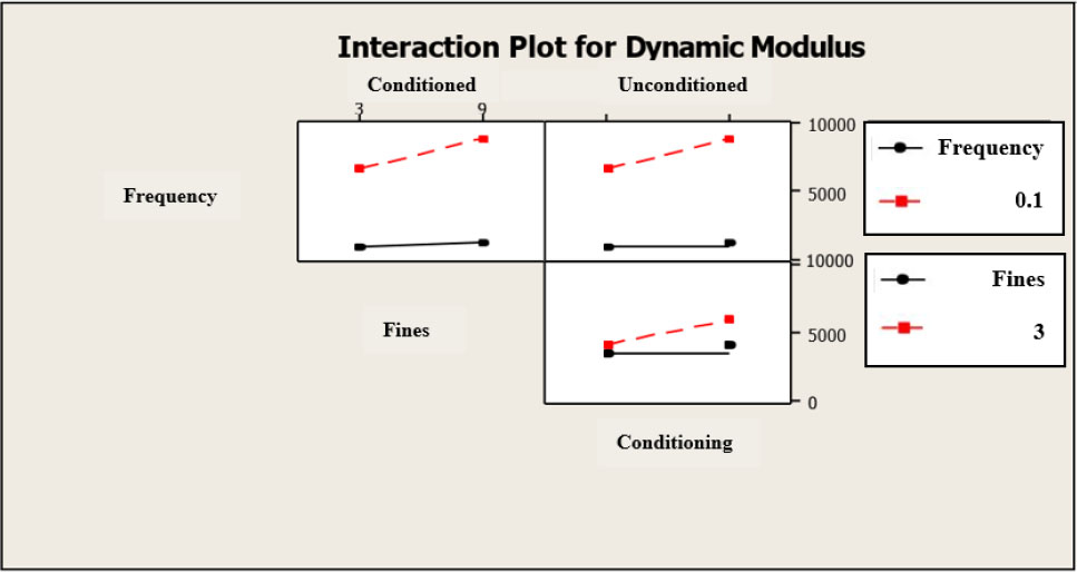
Figure 11.
Interaction plots for dynamic modulus.
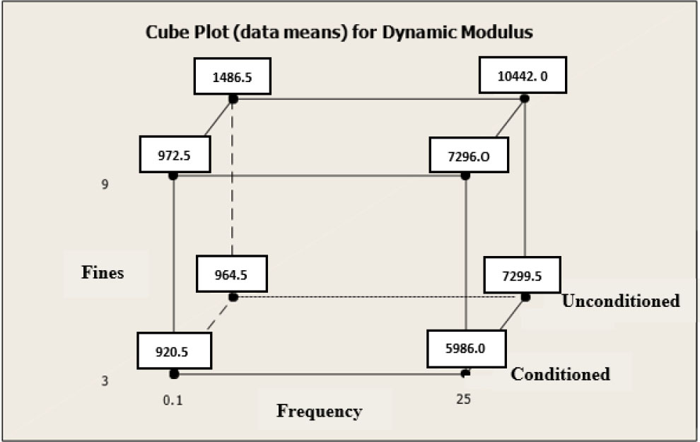
Figure 12:
Cube plot for dynamic modulus.
Table 7:
Analysis of variance for dynamic modulus.
| Sources | DF | SS | MSS | F-test | p-value |
|---|---|---|---|---|---|
| Main effects | 3 | 190,552,515 | 63,517,505 | 1336.0 | 0.000 |
| 2-way interactions | 3 | 8,892,063 | 2,964,021 | 62.35 | 0.000 |
| 3-way interactions | 1 | 464,442 | 464,442 | 9.77 | 0.014 |
| Residual error | 8 | 380,322 | 47,540 | ||
| Total | 1 | 200,289,341 | 47,540 |
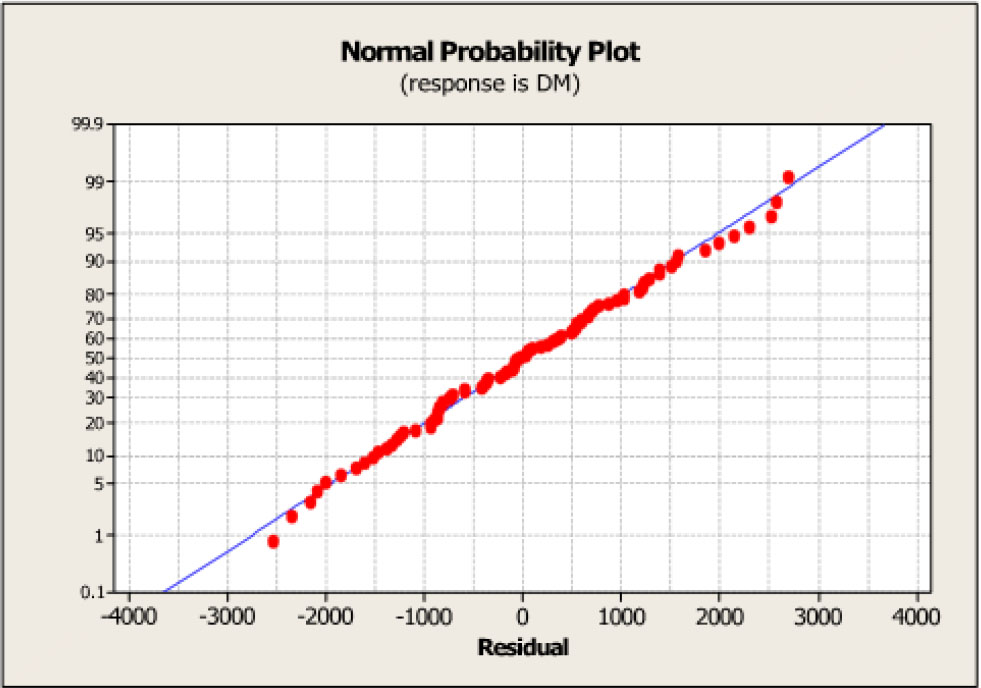
Figure 13:
Typical normal probability plot.
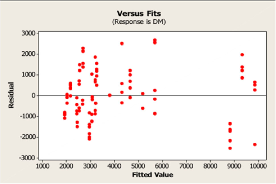
Figure 14:
Typical residual versus fitted values.
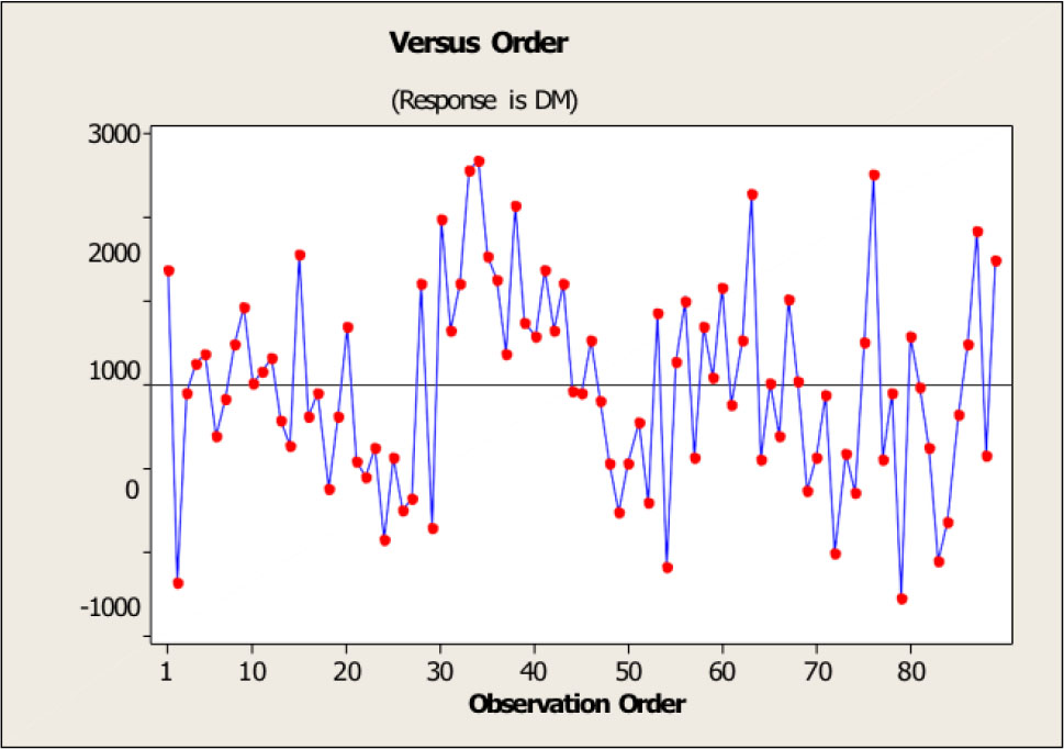
Figure 15:
Typical residual versus fitted values.
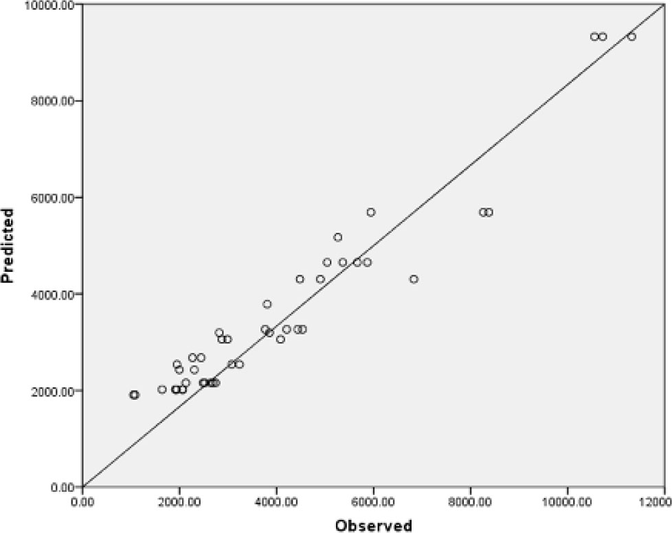
Figure 16:
Validation plot between predicted and observed values.