
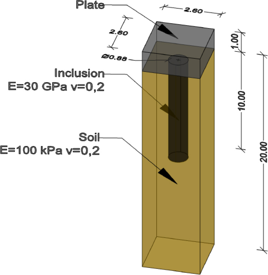
Figure 1:
Scheme of the reference problem.
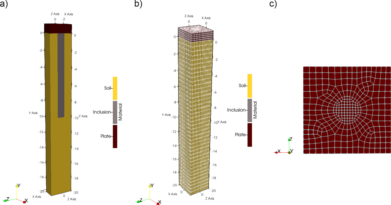
Figure 2:
Numerical model for Approach I: (a) model subdivision by type of continuum material; (b) finite element mesh-axonometric view; and (c) finite element mesh-top view.
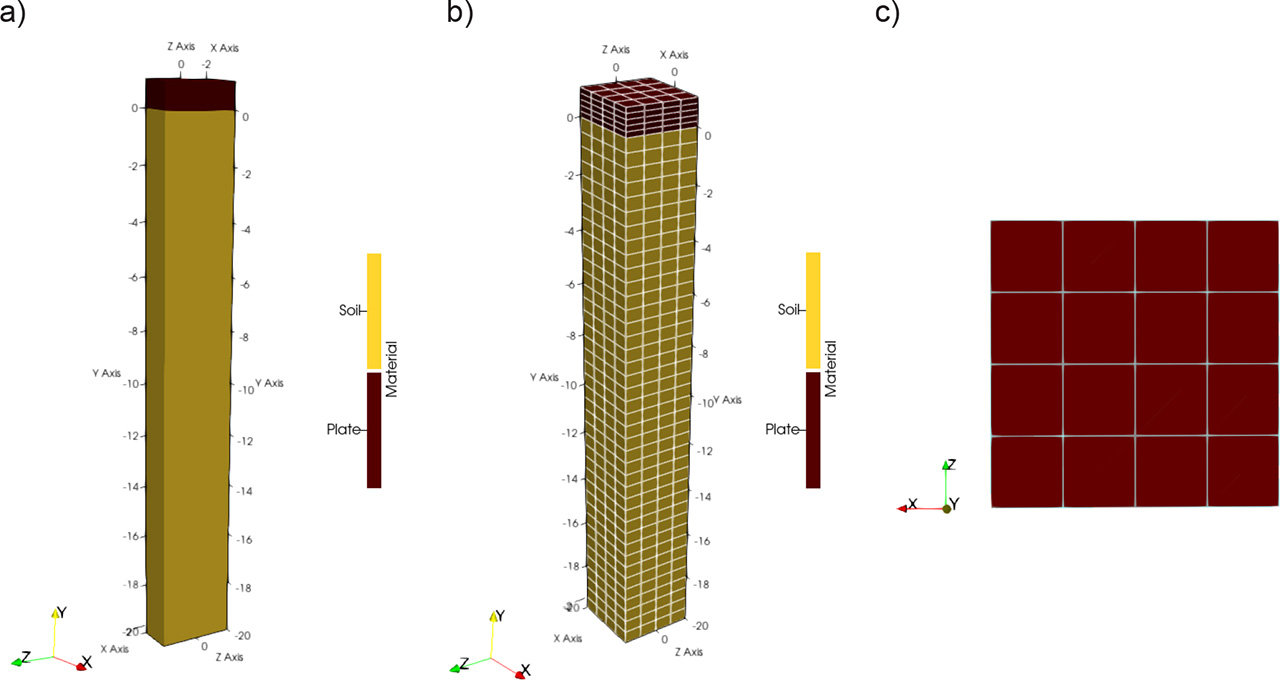
Figure 3:
Numerical model for Approach II: (a) model subdivision by the type of continuum material; (b) finite element mesh-axonometric view; and (c) finite element mesh-top view.
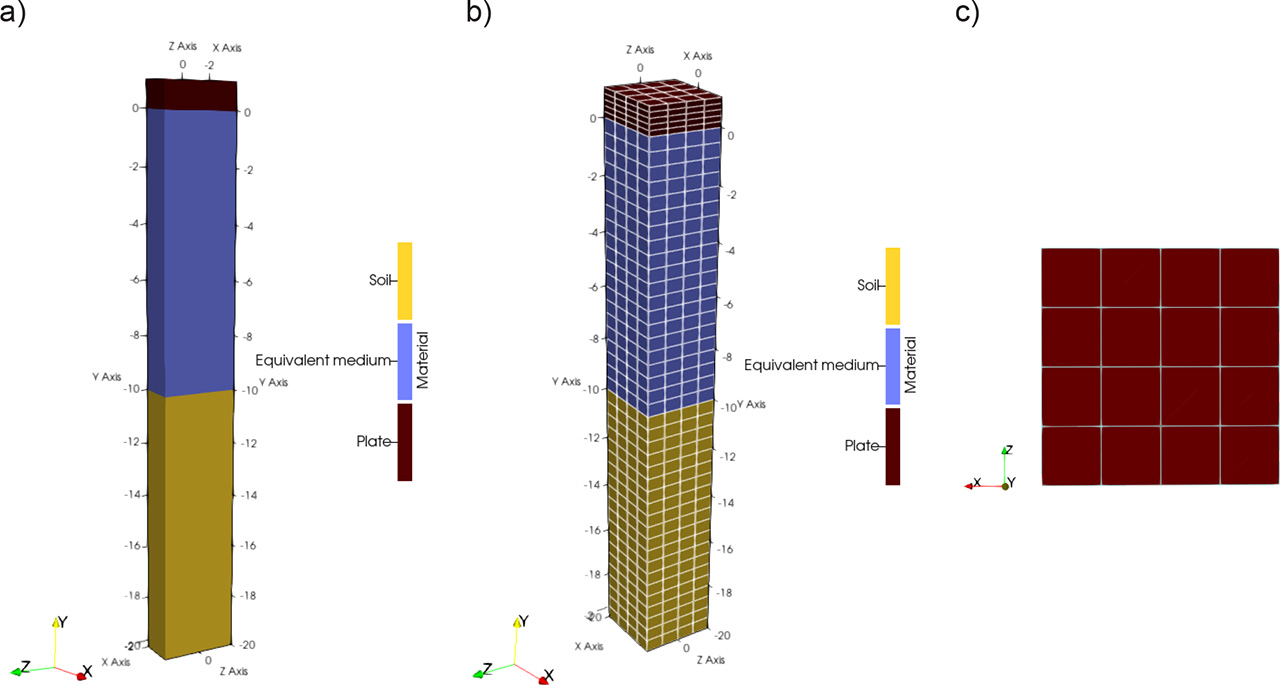
Figure 4:
Numerical model for Approach III: (a) model subdivision by the type of continuum material; (b) finite element mesh-axonometric view; and (c) finite element mesh-top view.
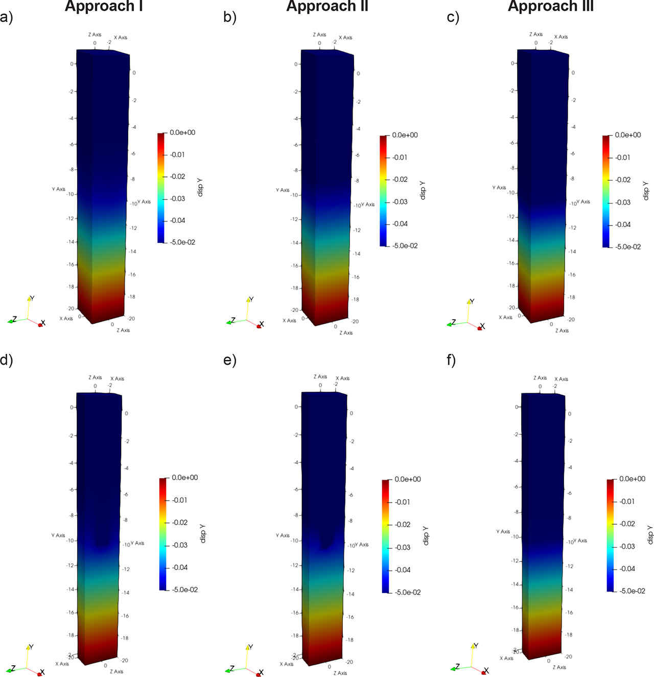
Figure 5:
Comparison of displacement maps according to selected design approaches.
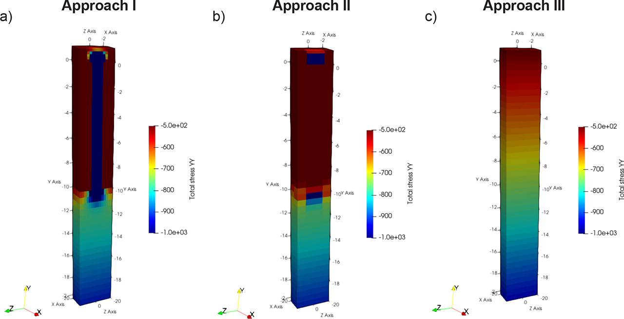
Figure 6:
Comparison of total vertical stress maps according to selected design approaches.
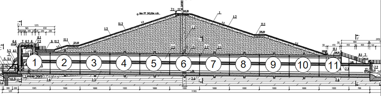
Figure 8:
Cross section through the dam.
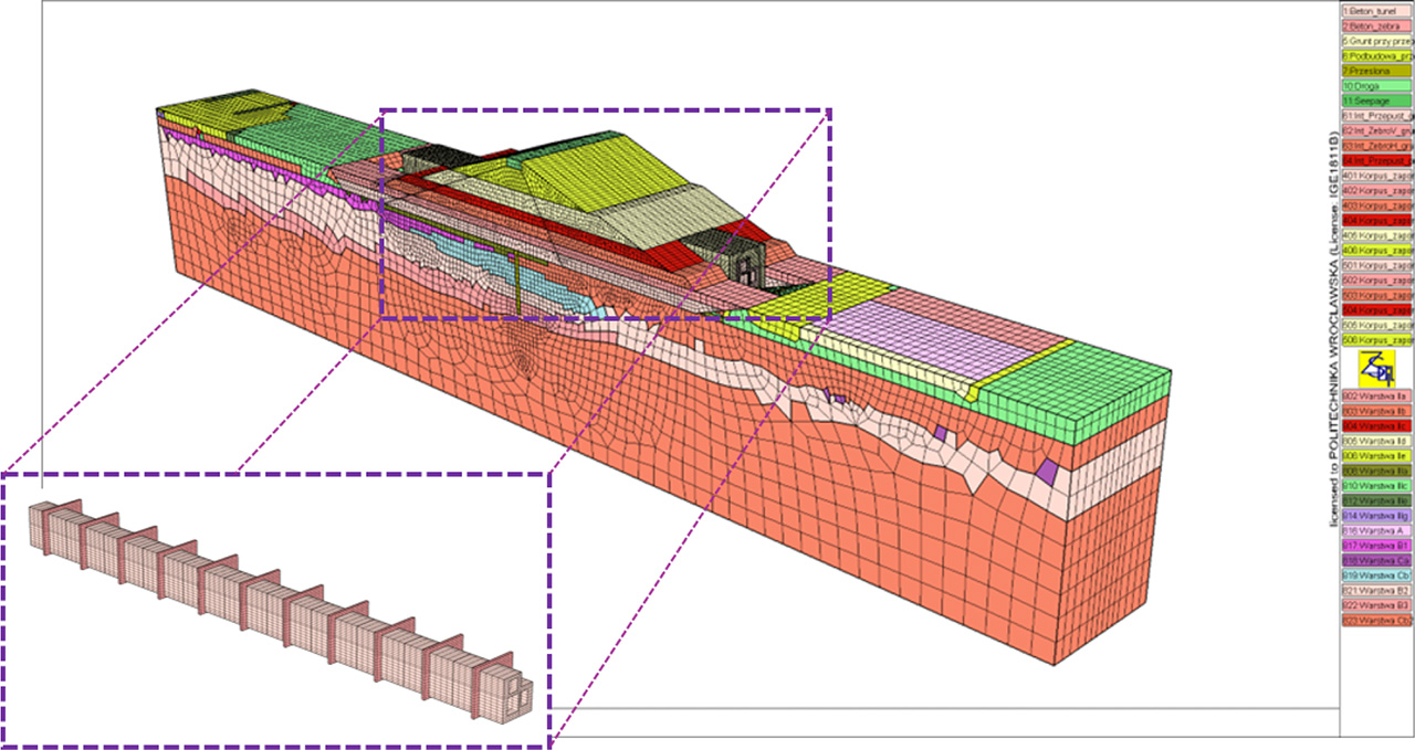
Figure 9:
Numerical model of the area under consideration.
Table 1:
List of geotechnical parameters for soils.
| Layer name | Soil type | Liquidity index/density index | Density ρ | Modulus Eo | Poisson ratio ν | Friction angle f | Cohesion c |
|---|---|---|---|---|---|---|---|
| - | - | - | g/cm3 | MPa | - | ° | kPa |
| Soils | |||||||
| IIc | siCl, saCl | IL<0.25 | 2.08 | 6.0 | 0.32 | 11 | 30 |
| IId | siCl, saCl | 0.25< IL <0.5 | 2.00 | 3.9 | 0.32 | 8 | 20 |
| IIe | siCl, saCl | 0.5< IL <1.0 | 1.98 | 3.6 | 0.32 | 6 | 10 |
| IIb | Gr, saGr | 0.33<ID<0.67 | 1.90 | 80 | 0.32 | 38 | 0 |
| IIa | MSa | 0.33<ID<0.67 | 1.75 | 60 | 0.32 | 32 | 0 |
| IIc | saCl | 0.25< IL <0.5 | 2.15 | 27 | 0.32 | 23 | 20 |
| IIf | grCl | 0.5< IL <1.0 | 2.12 | 9 | 0.32 | 18 | 10 |
| IIIa | Cl | IL <0 | 2.15 | 22 | 0.37 | 13 | 60 |
| IIIb | Cl | 0< IL <0.25 | 2.00 | 17 | 0.37 | 11 | 52 |
| IIIc | Cl | 0.25< IL <0.5 | 1.85 | 12 | 0.37 | 9 | 44 |
| Dam body | 2.20 | 55 | 0.32 | 33 | 0 | ||
| Impermeable core | 2.20 | 25 | 0.3 | 15 | 15 | ||
Table 2:
List of geotechnical parameters for rock layers.
| Rock layers adopted for computations | Depth range | Density P | Deformation modulus Eo | Poisson ratio ν | Friction angle □ | Cohesion c |
|---|---|---|---|---|---|---|
| - | m | g/cm3 | MPa | - | ° | kPa |
| A | - | 2.22 | 18 | 0.25 | 21.0 | 500 |
| B | <6 | 2.25 | 45 | 0.44 | 19.0 | 400 |
| B | 6–14 | 2.25 | 140 | 0.42 | 19.0 | 400 |
| B | >14 | 2.35 | 180 | 0.43 | 19.0 | 400 |
| Ca | - | 2.28 | 42 | 0.46 | 18.0 | 100 |
| Cb1 | <16 | 2.35 | 35 | 0.48 | 18.5 | 200 |
| Cb2 | >16 | 2.35 | 150 | 0.46 | 18.5 | 200 |
| Cc | - | 2.25 | 4 | 0.45 | 18.5 | 200 |
| D | - | 2.15 | 14 | 0.50 | 19.0 | 400 |
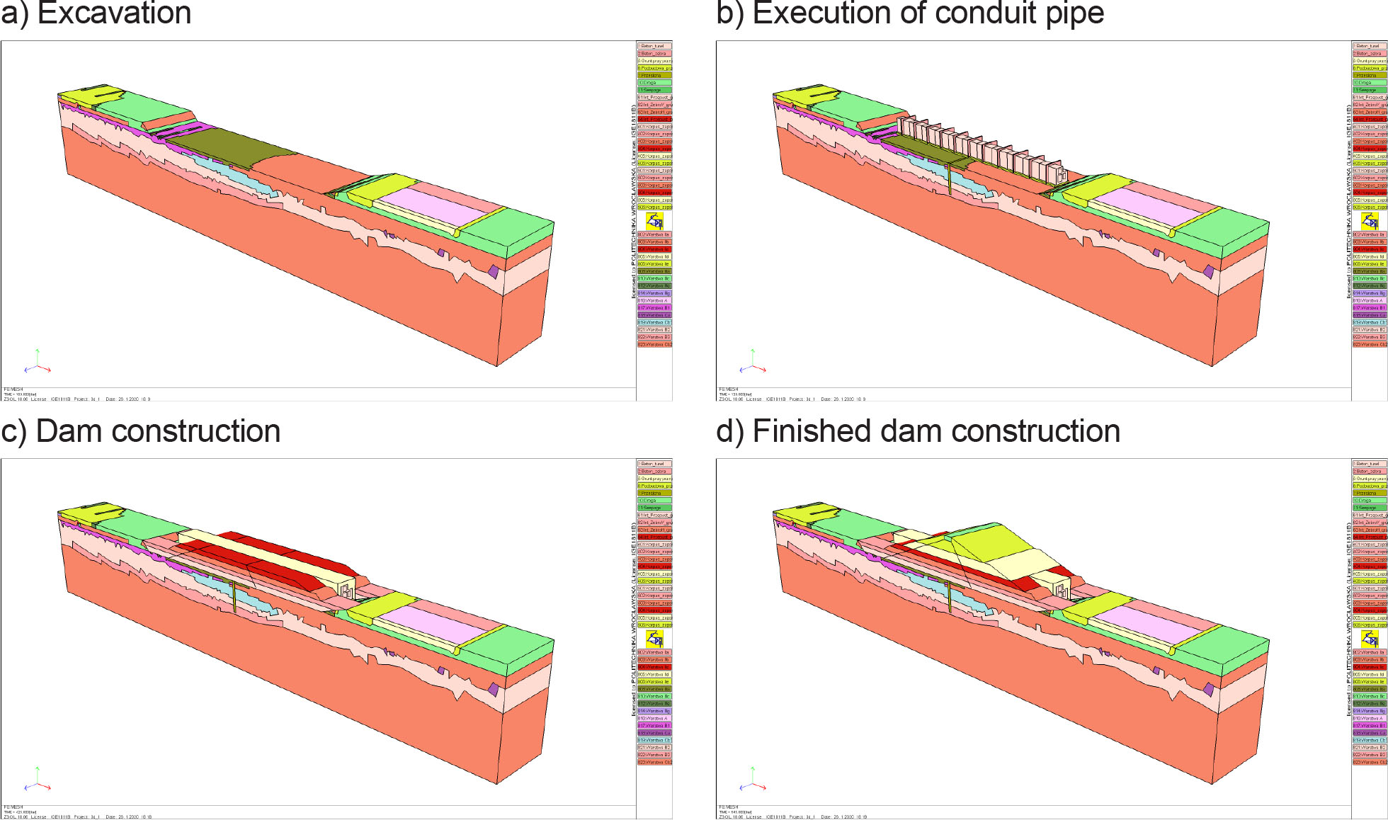
Figure 10:
Visualization of construction stages of the dam.
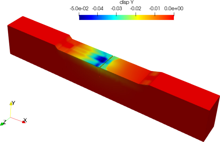
Figure 11:
Contour plot of vertical displacement at the foundation level of the conduit pipe.
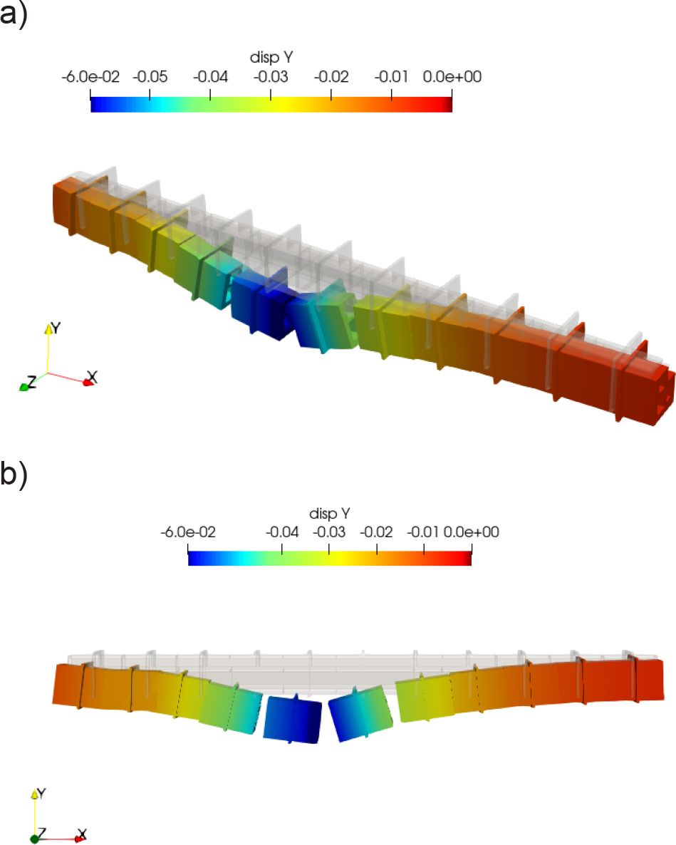
Figure 12:
Displacement Y of conduit on deformed mesh: (a) perspective view (b) side view.
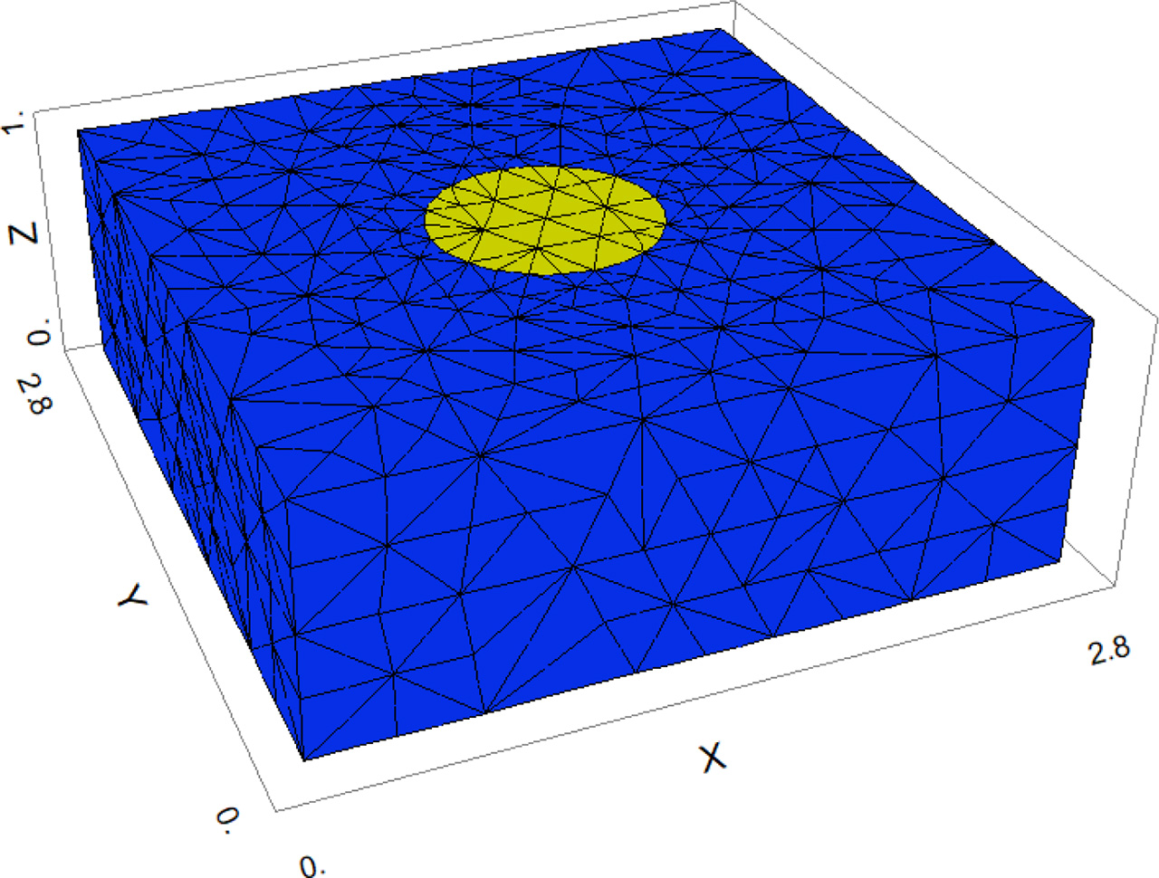
Figure 13:
An example view of the RVE model (yellow color – column, blue color – soil).
Table 3:
List of elastic parameters for soil without column with comparison to equivalent medium corresponding to specific soil with inclusion.
| Layer | Eo | ν | Eo, eff | νeff |
|---|---|---|---|---|
| - | MPa | - | MPa | - |
| IIIa | 22 | 0.37 | 2363 | 0.01 |
| B1 | 45 | 0.44 | 2457 | 0.05 |
| Cb1 | 35 | 0.48 | 2569 | 0.10 |
| B2 | 140 | 0.42 | 2624 | 0.09 |
| B3 | 180 | 0.43 | 2724 | 0.12 |
| Cb2 | 150 | 0.46 | 2796 | 0.17 |
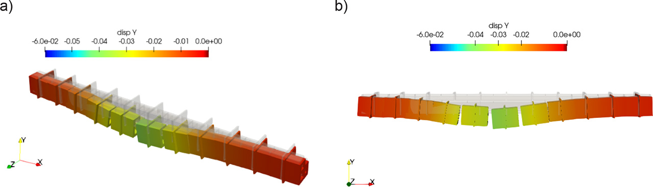
Figure 14:
Displacement Y of the conduit on the deformed mesh for Approach II: (a) perspective view (b) side view.
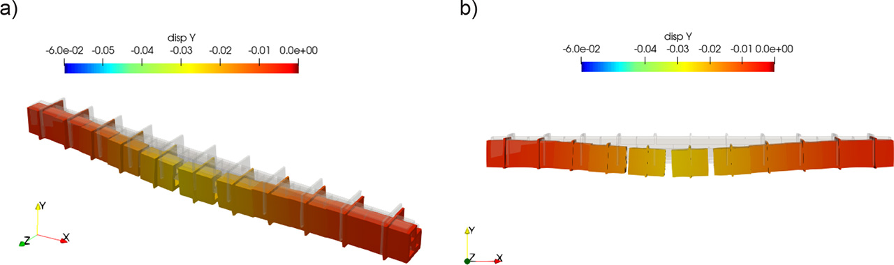
Figure 15:
Displacement Y of the conduit on the deformed mesh for Approach III: (a) perspective view and (b) side view.