
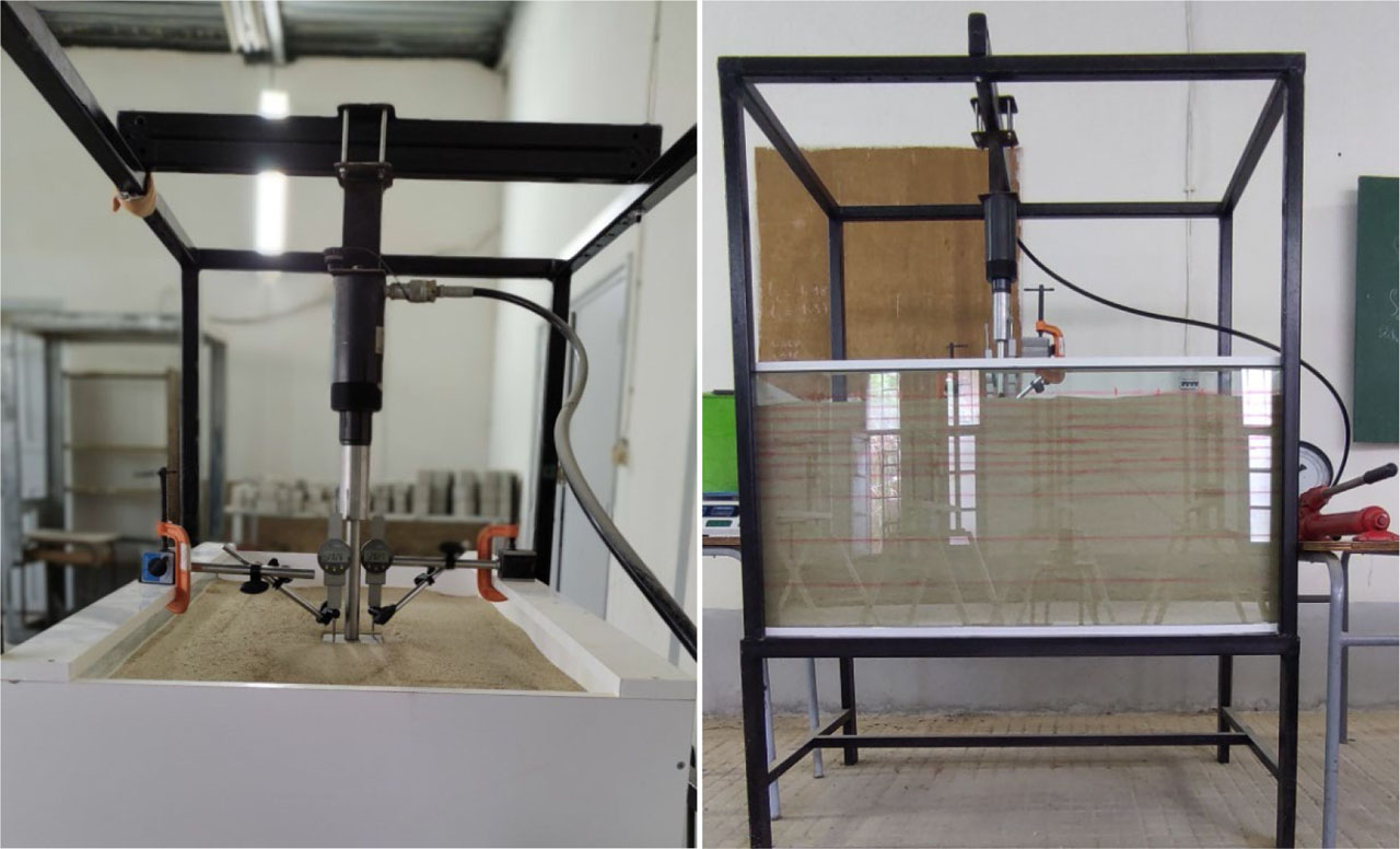
Figure 1:
View of the laboratory-scale model.
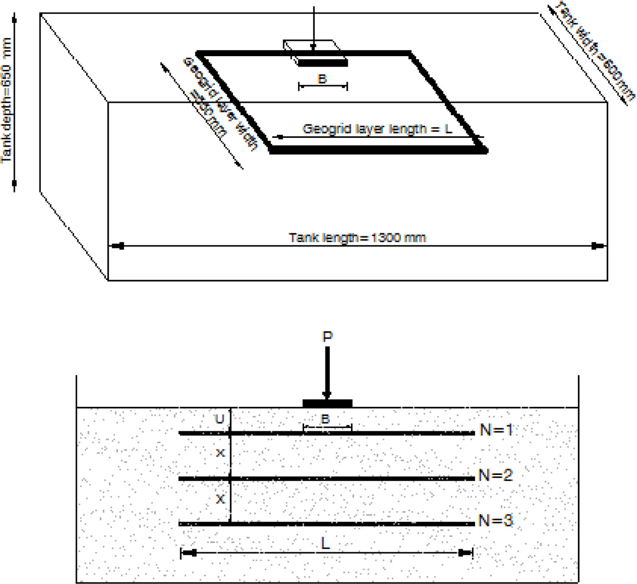
Figure 2:
Geometric model and studied parameters of the problem.
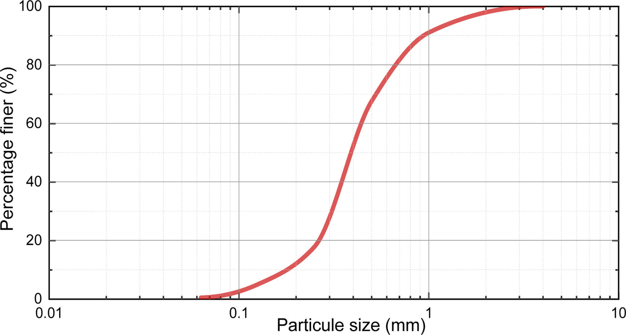
Figure 3:
Grain size curve of the testing material.
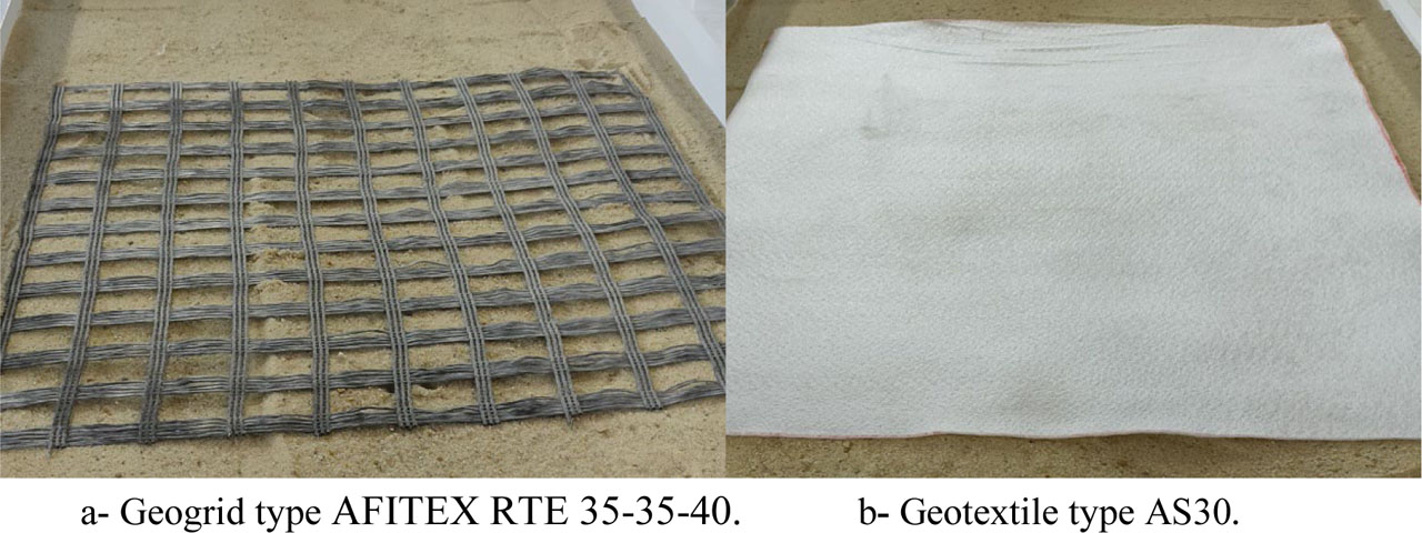
Figure 4:
Geosynthetic reinforcements used in this study.
Table 1:
Physical and mechanical properties of utilized reinforcement.
| Description | GeotextileAS30 | Geogrid AFITEX RTE 35–35–40 |
|---|---|---|
| - Total weight per unit area (g/m2) | 300.0 | 135.0 |
| - Thickness (mm) | 1.60 | - |
| - Mesh aperture size (mm) | - | 40×40 |
| - Peak tensile strength (kN/m) | 25.0 | 35.0 |
| - Extension at maximum load (%) | 75 | 10 |
| - CBR punching strength (kN) | 3.40 | - |
Table 2:
Levels of the input parameters used in the experimental design.
| Input parameters | Minimal value | Mean value | Maximal value |
|---|---|---|---|
| Length (L) | 5B | 7B | 9B |
| Number (N) | 1 | 2 | 3 |
| Depth of the first layer (U) | 0.25B | 0.5B | 0.75B |
| Spacing between layers (X) | 0.5B | 0.75B | 1.0B |
Table 3:
Experimental central composite design L25 of the current study.
| Run | Factor 1 L (*B) | Factor 2 N | Factor 3 U (*B) | Factor 4 X (*B) |
|---|---|---|---|---|
| 1 | 9 | 1 | 0.75 | 1 |
| 2 | 7 | 2 | 0.5 | 0.75 |
| 3 | 5 | 1 | 0.25 | 1 |
| 4 | 9 | 2 | 0,5 | 0.75 |
| 5 | 9 | 1 | 0.25 | 0.5 |
| 6 | 7 | 2 | 0.25 | 0.75 |
| 7 | 9 | 1 | 0.75 | 0.5 |
| 8 | 9 | 1 | 0.25 | 1 |
| 9 | 7 | 2 | 0.5 | 0.5 |
| 10 | 5 | 3 | 0.75 | 1 |
| 11 | 7 | 2 | 0.75 | 0.75 |
| 12 | 7 | 1 | 0.5 | 0.75 |
| 13 | 9 | 3 | 0.25 | 0.5 |
| 14 | 5 | 3 | 0.25 | 1 |
| 15 | 5 | 1 | 0.75 | 1 |
| 16 | 9 | 3 | 0.75 | 0.5 |
| 17 | 5 | 3 | 0.75 | 0.5 |
| 18 | 9 | 3 | 0.25 | 1 |
| 19 | 5 | 1 | 0.75 | 0.5 |
| 20 | 5 | 1 | 0.25 | 0.5 |
| 21 | 5 | 2 | 0.5 | 0.75 |
| 22 | 7 | 2 | 0.5 | 1 |
| 23 | 9 | 3 | 0.75 | 1 |
| 24 | 7 | 3 | 0.5 | 0.75 |
| 25 | 5 | 3 | 0.25 | 0.5 |
Table 4:
Experimental results for the two types of reinforcement.
| Run | Factor 1 L (*B) | Factor 2 N | Factor 3 U (*B) | Factor 4 X (*B) | Response 1 qGeogrid (kPa) | Response 2 qGeotextile(kPa) |
|---|---|---|---|---|---|---|
| 1 | 9 | 1 | 0.75 | 1 | 170.0 | 175.0 |
| 2 | 7 | 2 | 0.5 | 0.75 | 240.0 | 270.0 |
| 3 | 5 | 1 | 0.25 | 1 | 220 | 240 |
| 4 | 9 | 2 | 0.5 | 0.75 | 275 | 280 |
| 5 | 9 | 1 | 0.25 | 0.5 | 260 | 275 |
| 6 | 7 | 2 | 0.25 | 0.75 | 280 | 350 |
| 7 | 9 | 1 | 0.75 | 0.5 | 170 | 210 |
| 8 | 9 | 1 | 0.25 | 1 | 230 | 275 |
| 9 | 7 | 2 | 0.5 | 0.5 | 270 | 300 |
| 10 | 5 | 3 | 0.75 | 1 | 160 | 210 |
| 11 | 7 | 2 | 0.75 | 0.75 | 165 | 190 |
| 12 | 7 | 1 | 0.5 | 0.75 | 180 | 200 |
| 13 | 9 | 3 | 0.25 | 0.5 | 360 | 450 |
| 14 | 5 | 3 | 0.25 | 1 | 350 | 485 |
| 15 | 5 | 1 | 0.75 | 1 | 140 | 165 |
| 16 | 9 | 3 | 0.75 | 0.5 | 165 | 180 |
| 17 | 5 | 3 | 0.75 | 0.5 | 170 | 165 |
| 18 | 9 | 3 | 0.25 | 1 | 300 | 420 |
| 19 | 5 | 1 | 0.75 | 0.5 | 140 | 160 |
| 20 | 5 | 1 | 0.25 | 0.5 | 220 | 240 |
| 21 | 5 | 2 | 0.5 | 0.75 | 245 | 260 |
| 22 | 7 | 2 | 0.5 | 1 | 200 | 240 |
| 23 | 9 | 3 | 0.75 | 1 | 180 | 185 |
| 24 | 7 | 3 | 0.5 | 0.75 | 280 | 370 |
| 25 | 5 | 3 | 0.25 | 0.5 | 395 | 525 |
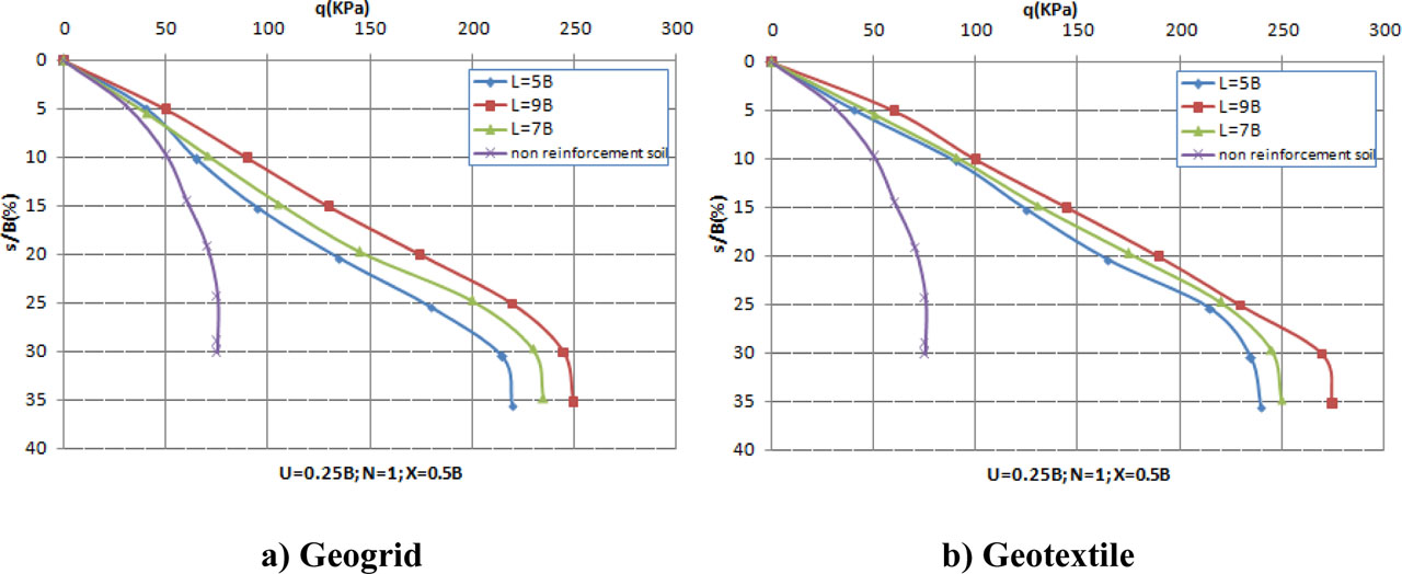
Figure 5:
Effect of length on q – s/B relationship (U=0.25B, N=1, X=0.5B).
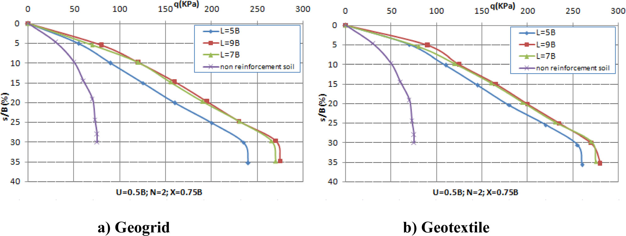
Figure 6:
Effect of length on q–s/B relationship (U=0.5B, N=2, X=0.75B).
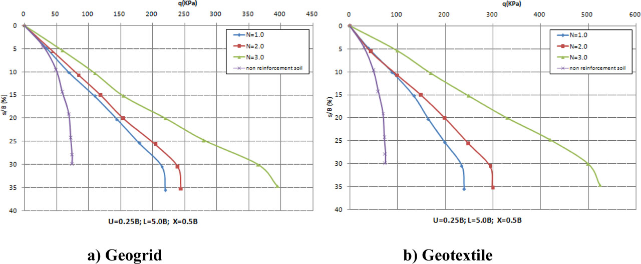
Figure 7:
Effect of reinforcement number on q–s/B relationship (U=0.25B, L=5.0B, X=0.5B).
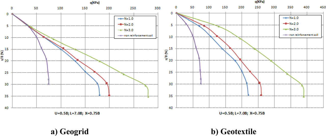
Figure 8:
Effect of reinforcement number on q–s/B relationship (U=0.5B, L=7.0B, X=0.75B).
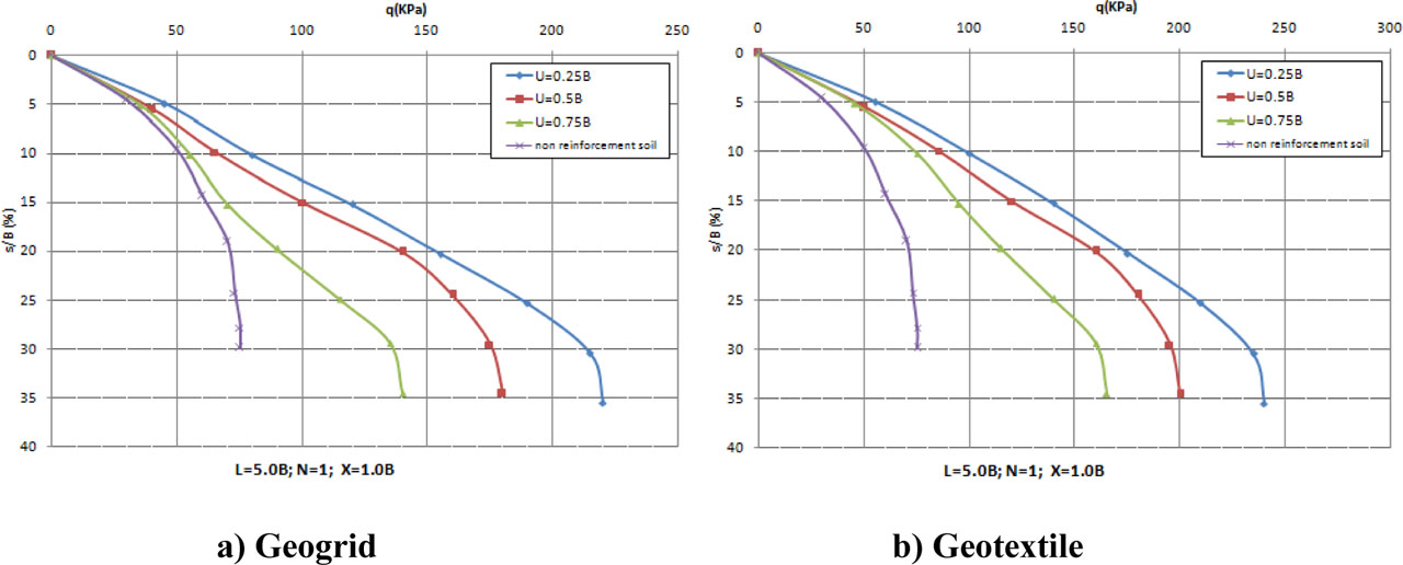
Figure 9:
Effect of the depth of the first layer on q–s/B relationship (L=5.0B, N=1, X=1.0B).
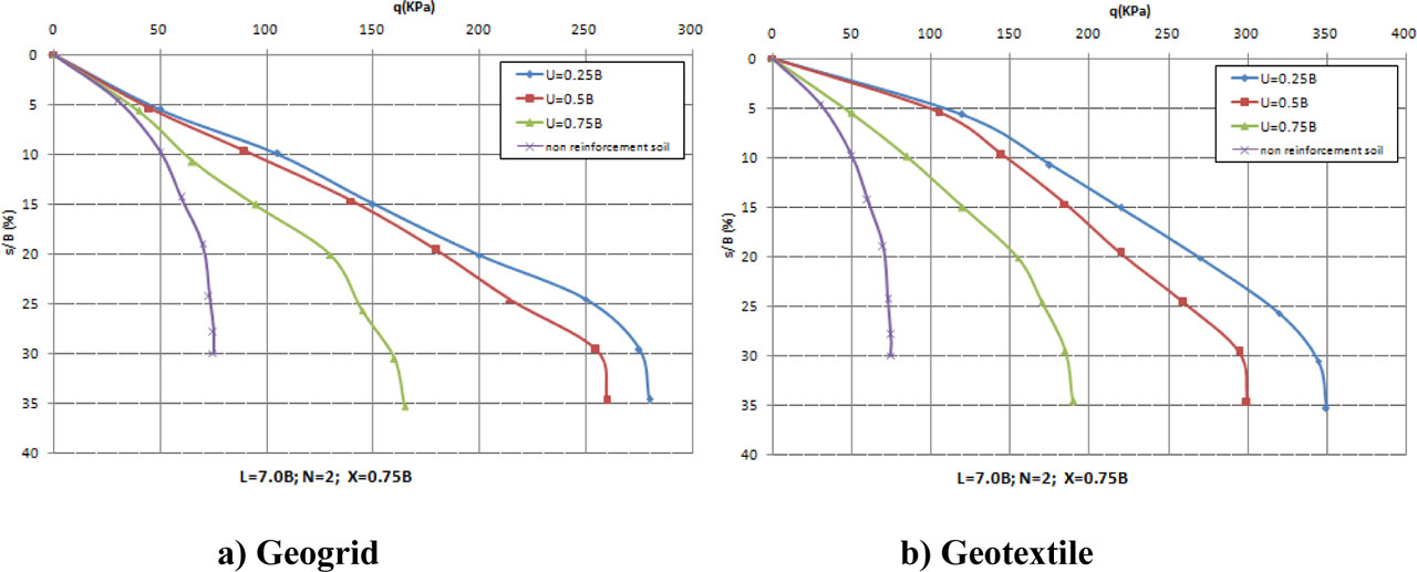
Figure 10:
Effect of the depth of the first layer on q–s/B relationship (L=7.0B, N=2, X=0.75B).
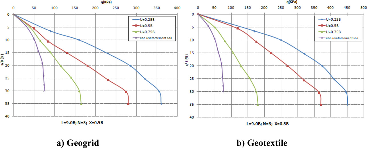
Figure 11:
Effect of the depth of the first layer on q–s/B relationship (L=9.0B, N=3, X=0.5B).
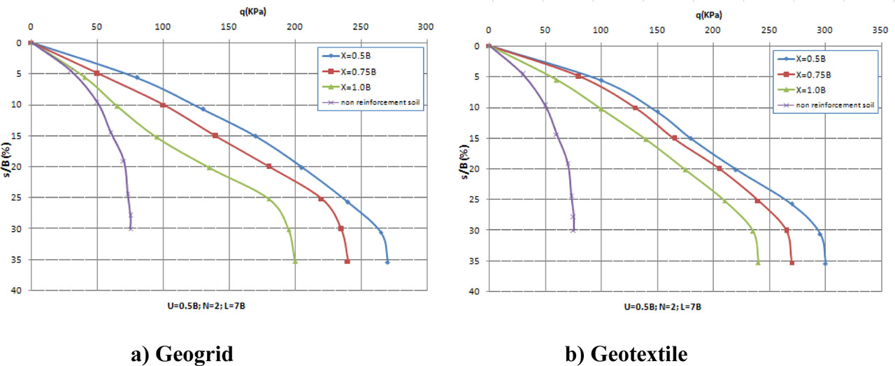
Figure 12:
Effect of the spacing reinforcement on q–s/B relationship (U=0.5B, N=2, L=7.0B).
Table 5:
ANOVA results of the bearing capacity for geogrid reinforcement.
| Source | Sum of squares | Df | Mean square | F value | P-value Prob> F | Cont (%) | Remark |
|---|---|---|---|---|---|---|---|
| Model | 1.156E+005 | 11 | 10,512.06 | 40.30 | < 0.0001 | Significant | |
| L (length of layers) | 272.22 | 1 | 272.22 | 1.04 | 0.3256 | 0.234 | Insignificant |
| N (number of layers) | 22,050.00 | 1 | 22,050.00 | 84.52 | < 0.0001 | 18.970 | Significant |
| U (depth of the first layer) | 74,112.50 | 1 | 74,112.50 | 284.10 | < 0.0001 | 63.762 | Significant |
| X (spacing between layers) | 1605.56 | 1 | 1605.56 | 6.15 | 0.0276 | 1.381 | Significant |
| L*N | 2025.00 | 1 | 2025.00 | 7.76 | 0.0154 | 1.742 | Significant |
| L*U | 756.25 | 1 | 756.25 | 2.90 | 0.1124 | 0.651 | Insignificant |
| N*U | 11,025.00 | 1 | 11,025.00 | 42.26 | < 0.0001 | 9.485 | Significant |
| U*X | 1225.00 | 1 | 1225.00 | 4.70 | 0.0494 | 1.054 | Significant |
| L2 | 1303.60 | 1 | 1303.60 | 5.00 | 0.0436 | 1.122 | Significant |
| U2 | 681.69 | 1 | 681.69 | 2.61 | 0.1300 | 0.586 | Insignificant |
| X2 | 915.48 | 1 | 915.48 | 3.51 | 0.0837 | 0.788 | Insignificant |
| Residual | 3391.33 | 13 | 260.87 | 0.224 | Insignificant | ||
| Cor total | 1.190E+005 | 24 |
Table 6:
ANOVA results of the bearing capacity for geotextile reinforcement.
| Source | Sum of squares | Df | Mean square | F value | P-value Prob> F | Cont (%) | Remark |
|---|---|---|---|---|---|---|---|
| Model | 2.601E+005 | 11 | 23,641.60 | 28.90 | < 0.0001 | Significant | |
| L (length of layers) | 1.39 | 1 | 1.39 | 1.698E-003 | 0.9678 | 0.001 | Insignificant |
| N (number of layers) | 61,250.00 | 1 | 61,250.00 | 74.86 | < 0.0001 | 23.439 | Significant |
| U (depth of the first layer) | 1.458E+005 | 1 | 1.458E+005 | 178.20 | < 0.0001 | 55.795 | Significant |
| X (spacing between layers) | 1422.22 | 1 | 1422.22 | 1.74 | 0.2101 | 0.544 | Insignificant |
| L*N | 4900.00 | 1 | 4900.00 | 5.99 | 0.0294 | 1.875 | Significant |
| L*U | 900.00 | 1 | 900.00 | 1.10 | 0.3134 | 0.344 | Insignificant |
| N*U | 42,025.00 | 1 | 42,025.00 | 51.36 | < 0.0001 | 16.082 | Significant |
| U*X | 506.25 | 1 | 506.25 | 0.62 | 0.4456 | 0.194 | Insignificant |
| L2 | 881.50 | 1 | 881.50 | 1.08 | 0.3182 | 0.337 | Insignificant |
| U2 | 1144.99 | 1 | 1144.99 | 1.40 | 0.2580 | 0.438 | Insignificant |
| X2 | 1666.27 | 1 | 1666.27 | 2.04 | 0.1771 | 0.638 | Insignificant |
| Residual | 10,636.42 | 13 | 818.19 | 0.313 | Insignificant | ||
| Cor total | 2.707E+005 | 24 |
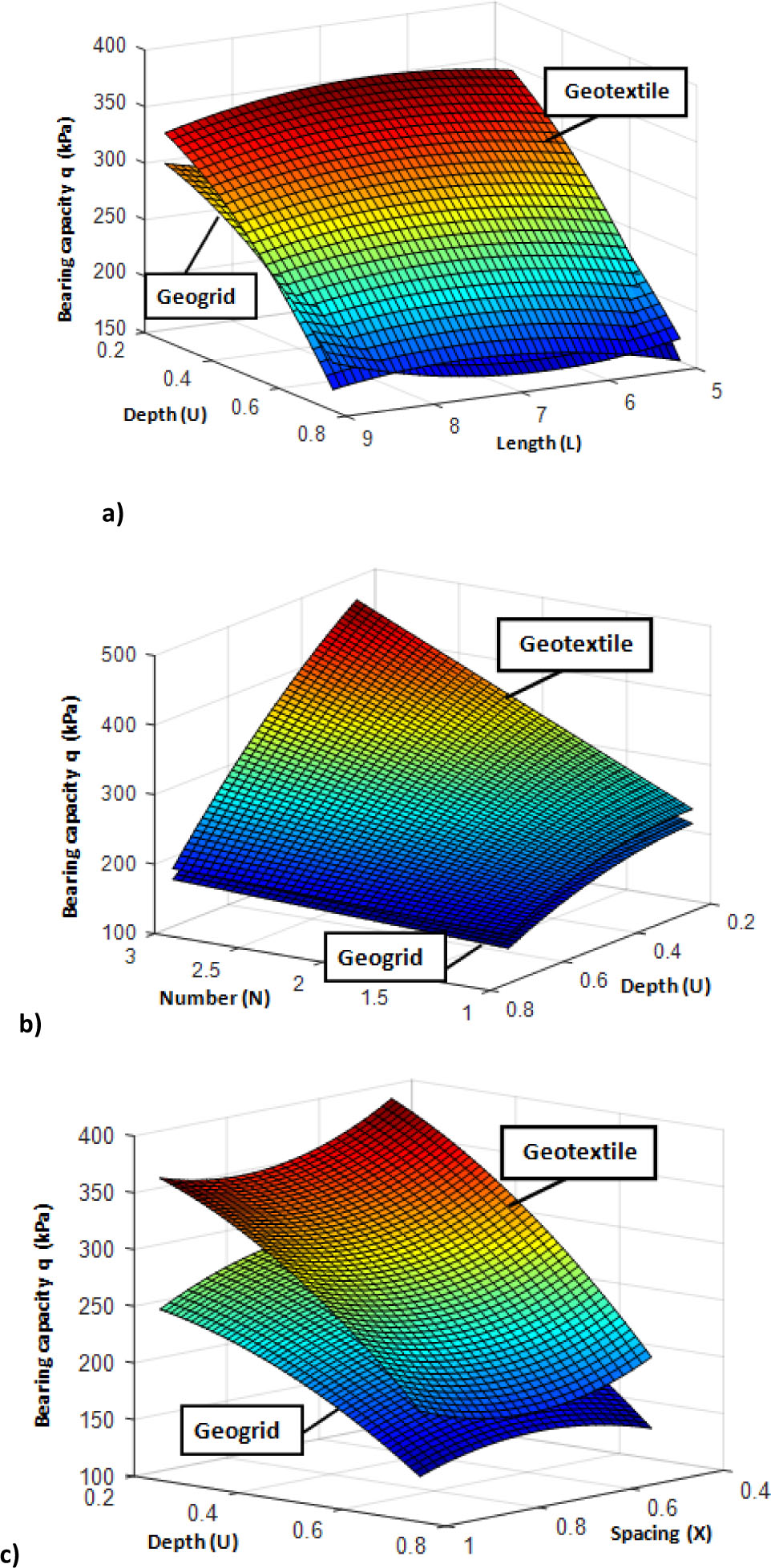
Figure 13:
Effect of geometric parameters on the bearing capacity for the three soils.
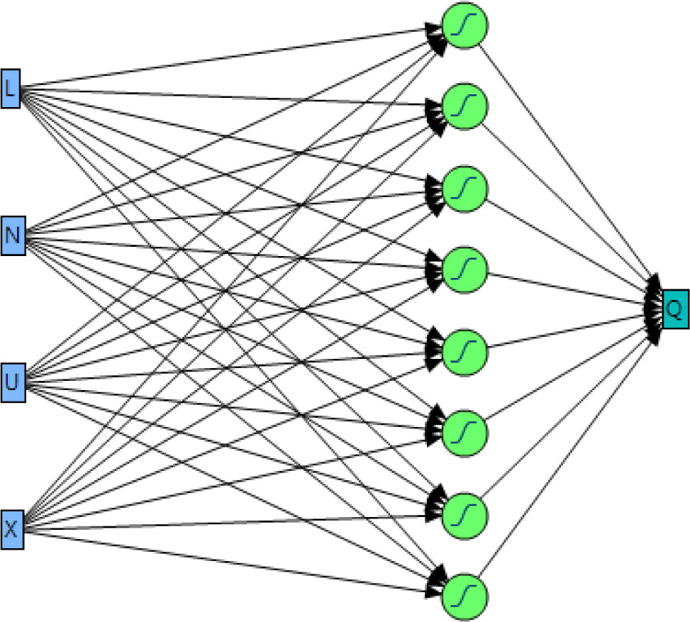
Figure 14:
ANN architecture (4 -8 -1) for bearing capacity q.
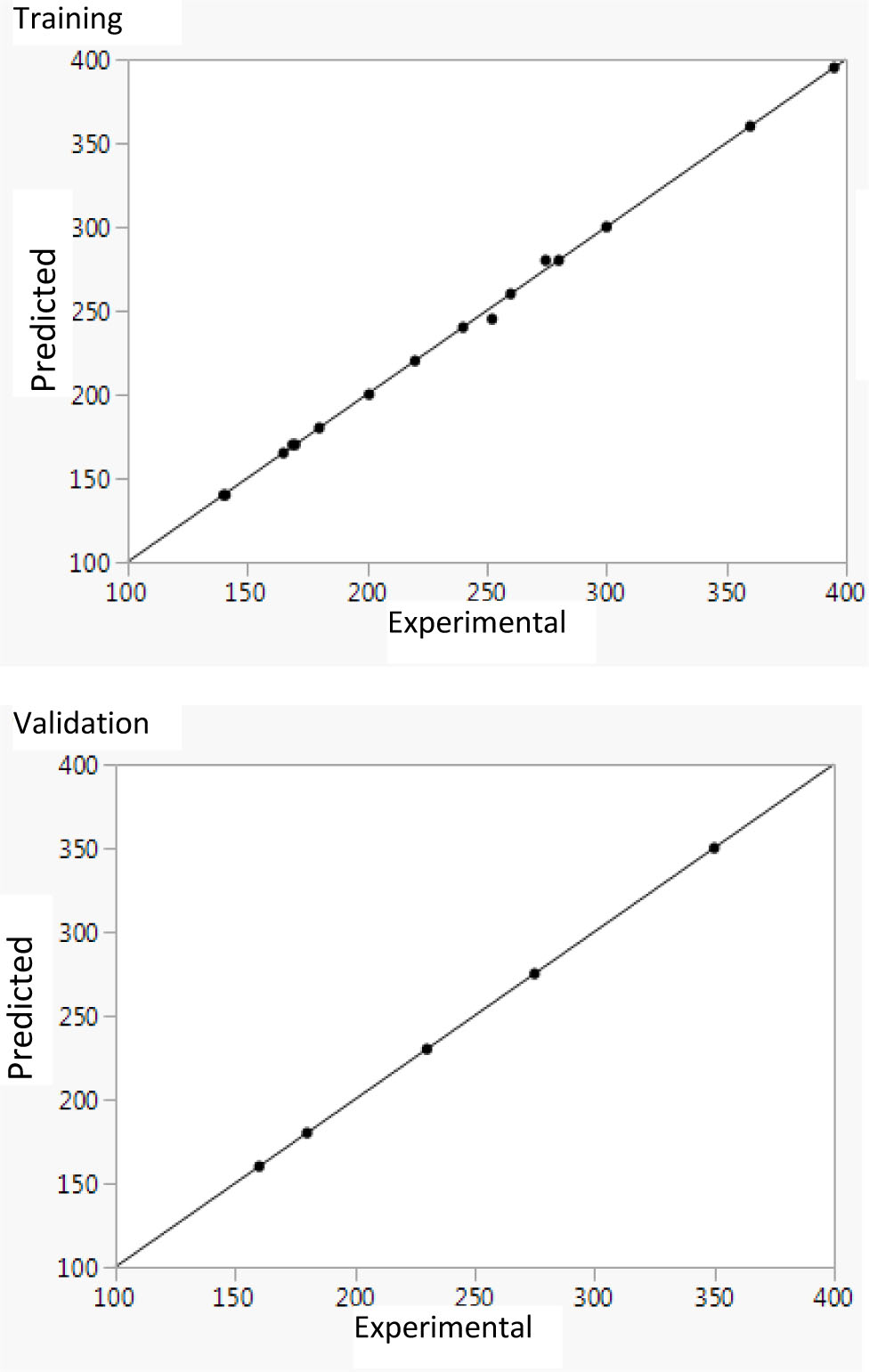
Figure 15:
Predicted versus experimental values for bearing capacity q.
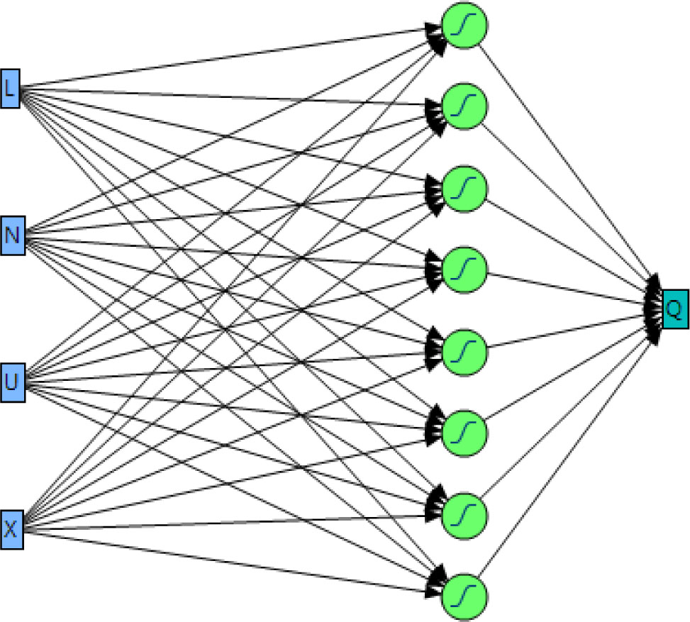
Figure 16:
ANN architecture (4 -8 -1) for the bearing capacity q.
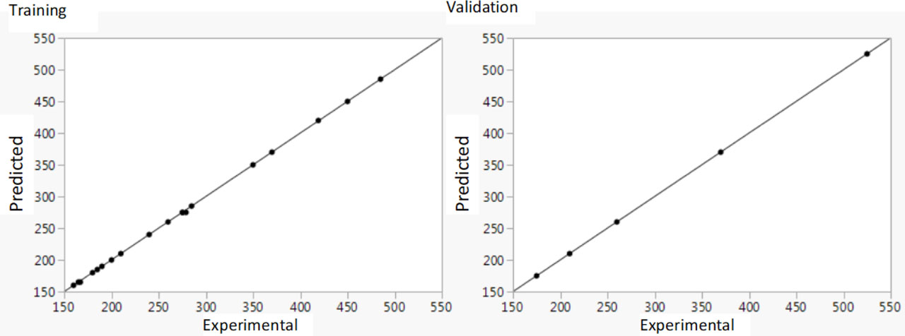
Figure 17:
Predicted versus experimental values for the bearing capacity q.
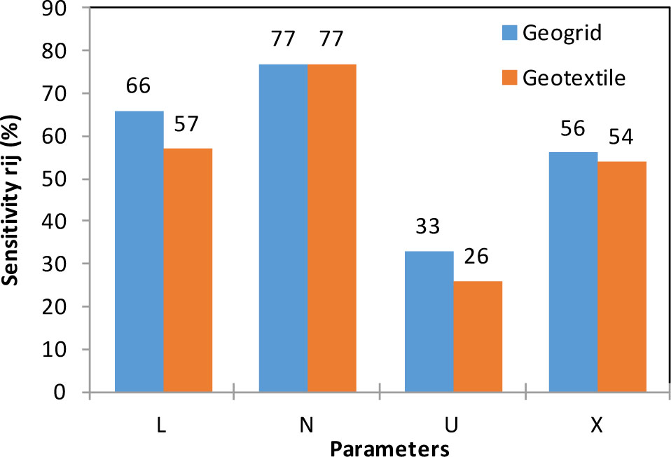
Figure 18:
Results of sensitivity analysis using CAM.
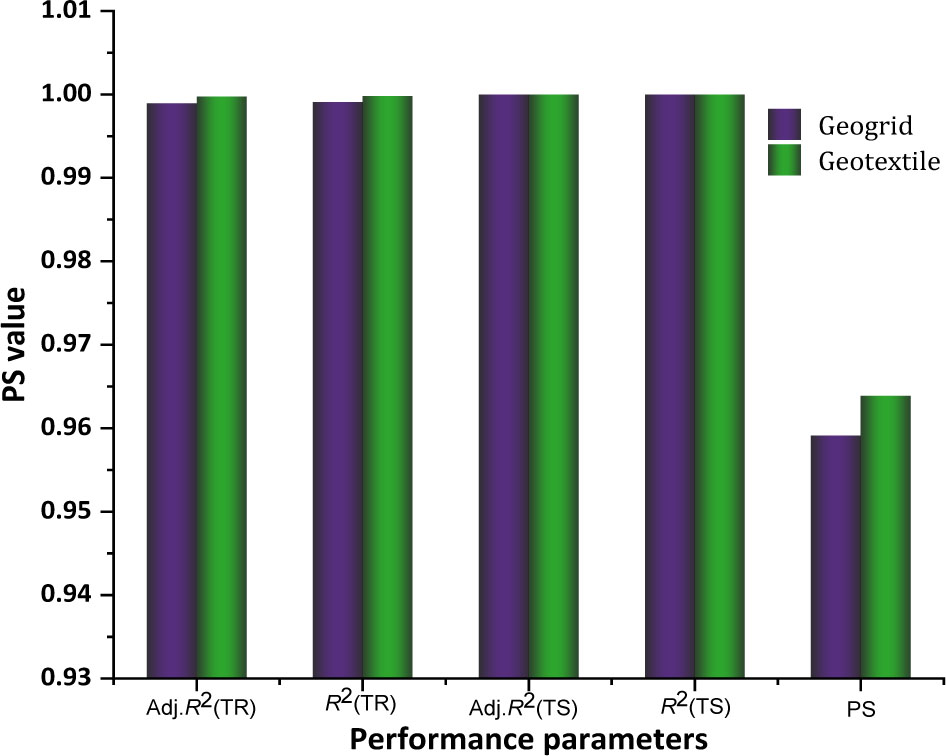
Figure 19:
Bar plot of PS values.
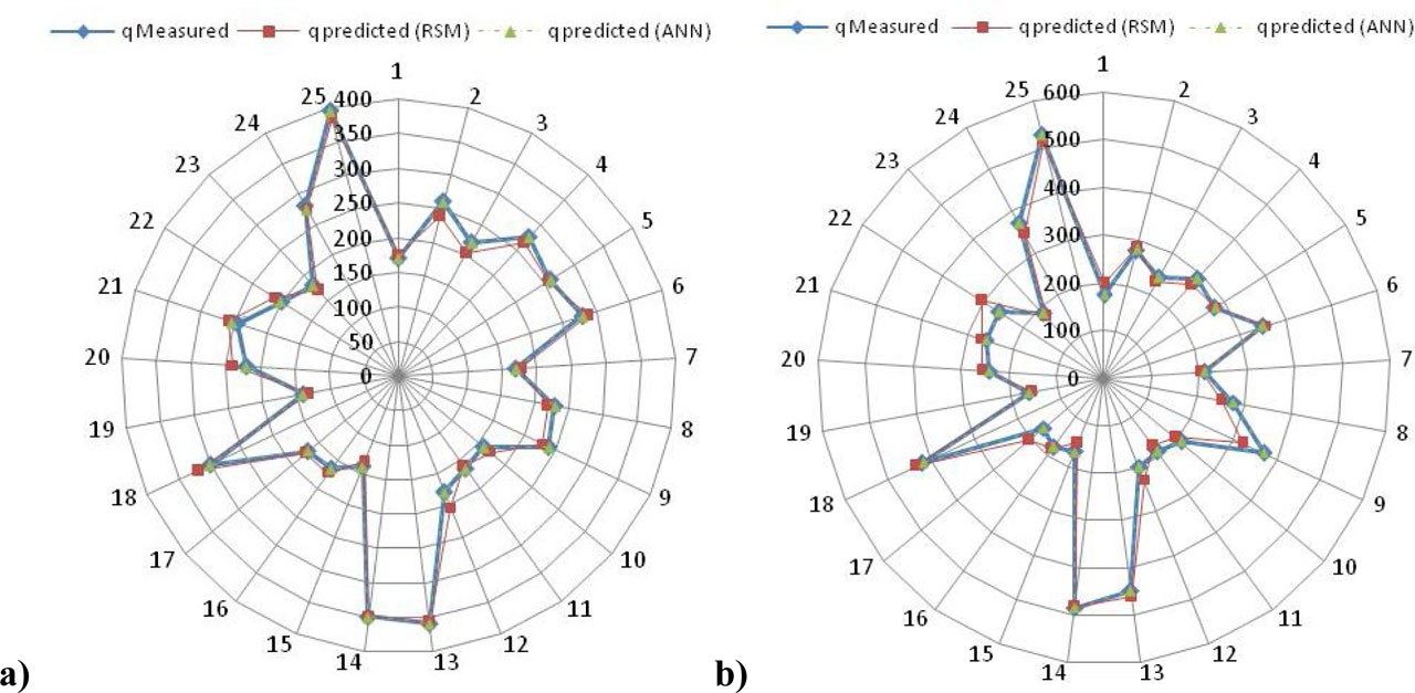
Figure 20:
Comparison between predicted and experimental values for q with RSM and ANN models (a- geogrid reinforcement. b- geotextile reinforcement).
Table 7:
Comparison between RSM and ANN models.
| Type of reinforcement | RSM | ANN | ||||
|---|---|---|---|---|---|---|
| R2 | RMSE | MPE (%) | R2 | RMSE | MPE (%) | |
| Geogrid | 0.972 | 0.3595 | 0.7215 | 0.9991 | 0.057 | 0.0414 |
| Geotextile | 0.961 | 0.6366 | 1.027 | 0.9998 | 0.0286 | 0.021 |
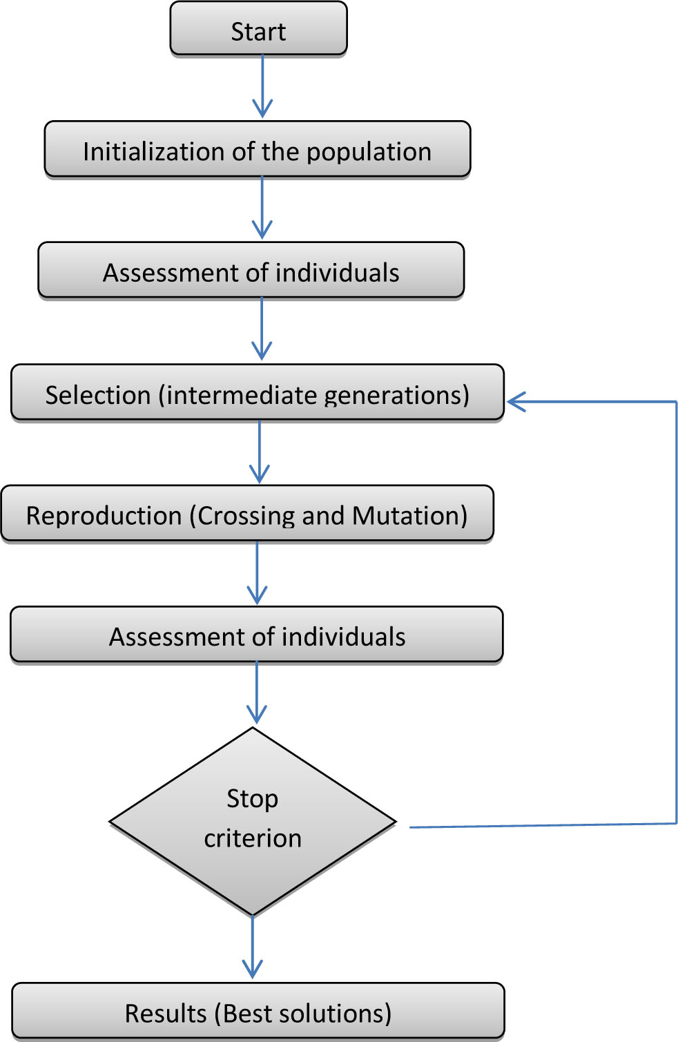
Figure 21:
Diagram of the genetic algorithm.
Table 8:
Optimization conditions.
| Parameters | Objective | Lower limit | Upper limit | |
|---|---|---|---|---|
| L (B) | Is in range | 5.0 | 9.0 | |
| N | Is in range | 1 | 3 | |
| U (B) | Is in range | 0.25 | 0.75 | |
| X(B) | Is in range | 0.5 | 1.0 | |
| q (kPa) | Geogrid | Maximization | 140.0 | 395.0 |
| Geotextile | 160.0 | 525.0 | ||
| Cost (B) | Minimization | 5.25 | 29.75 | |