
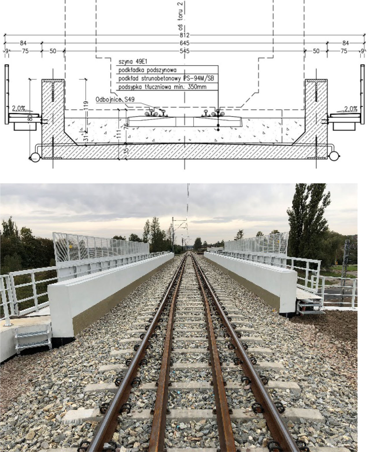
Figure 1
Dąbrowa bridge (picture by Nowak MOSTY).
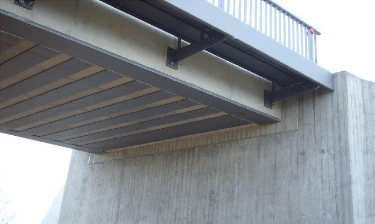
Figure 2
The idea of external reinforcement by SSF Ingenieure applied in the trough girders (both in the longitudinal and transversal directions of the slab for railway bridges) in the bridge located next to Spergau [9, 1] (picture by Guenter Seidl).
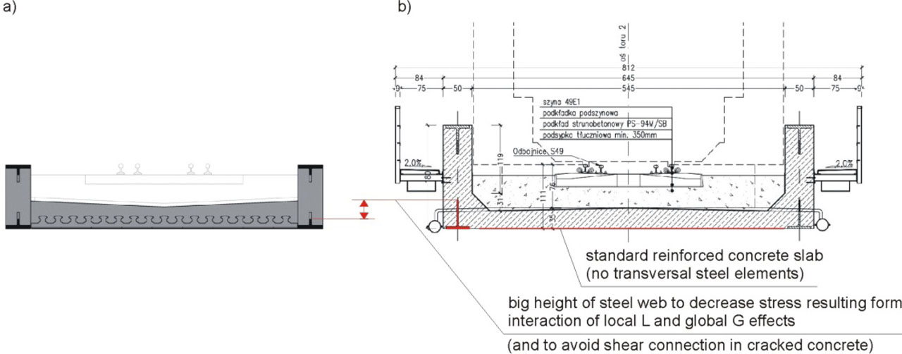
Figure 3
The main differences between 13 m span bridge next to Spergau by “SSF Ingenieure” design office and 23 m bridge in Dąbrowa Górnicza by “FASYS Mosty” design office (reinforced concrete slab and enlarged height of webs of T-sections): a) bridge by SSF using external reinforcement, b) bridge in Dąbrowa Górnicza using general composite section.
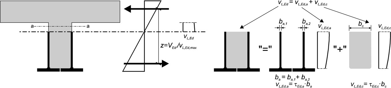
Figure 4
Distribution of longitudinal shear in a combined general composite section [3].
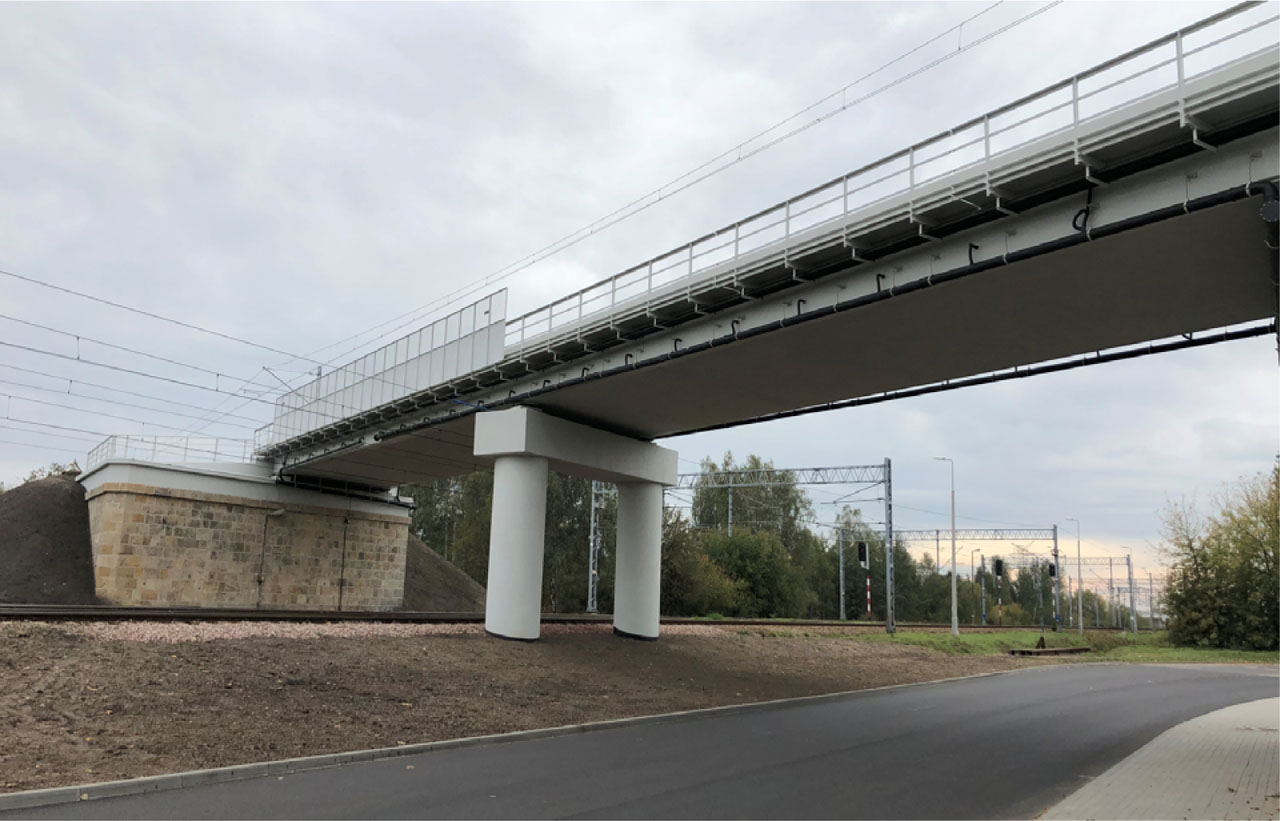
Figure 5
General view of the bridge (picture by Nowak Mosty).
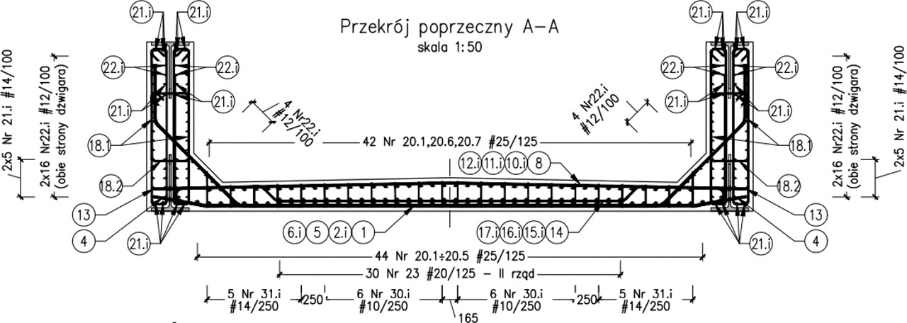
Figure 6
Reinforcing bars in cross section [57].
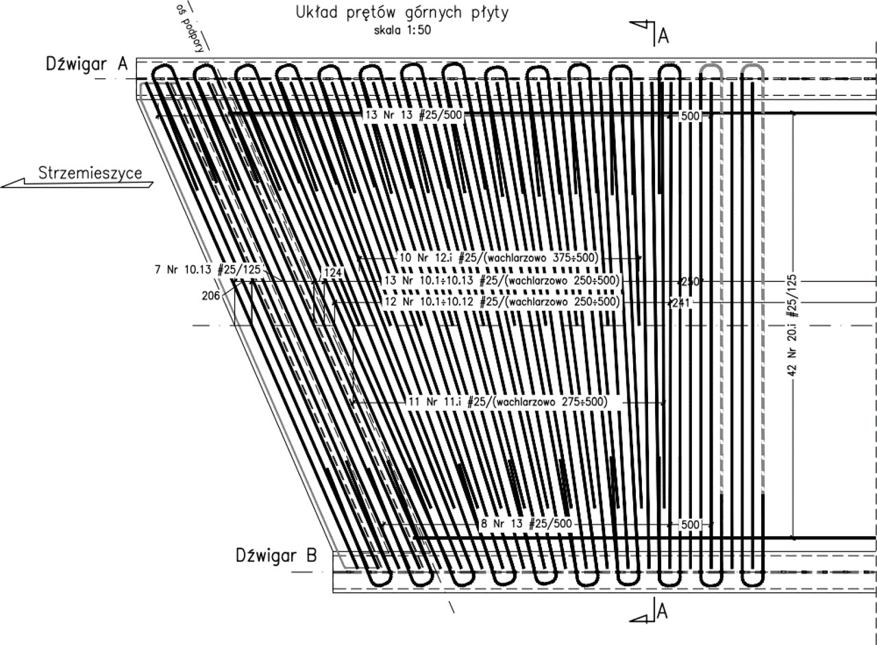
Figure 7
Upper reinforcement in slab [57].
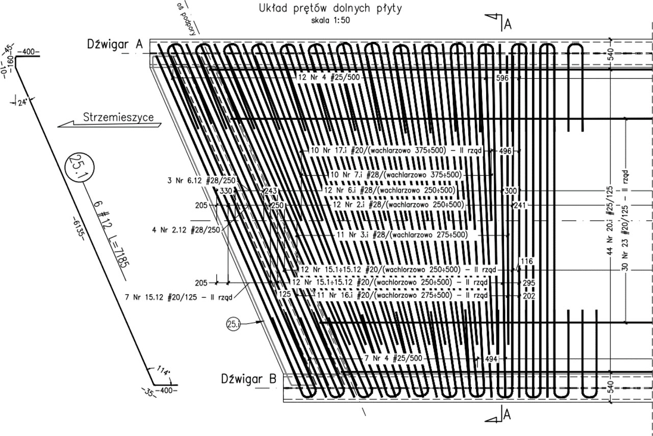
Figure 8
Bottom reinforcement in slab [57].
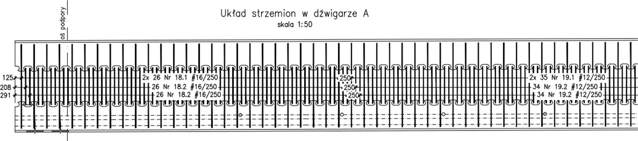
Figure 9
Shear reinforcement of hybrid girders [57].
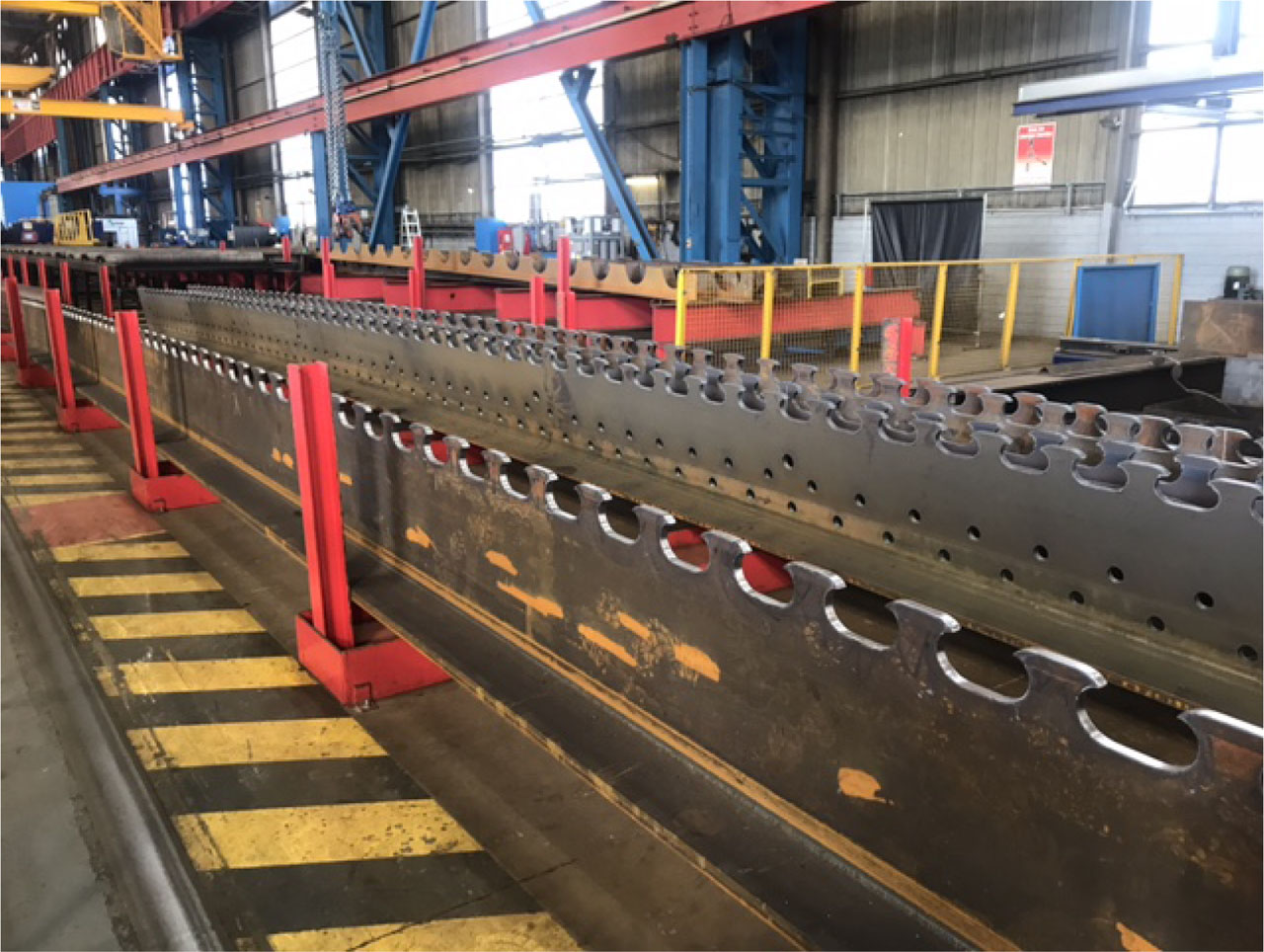
Figure 10
Steel T-sections produced in Luxembourg (picture: ArcelorMittal).
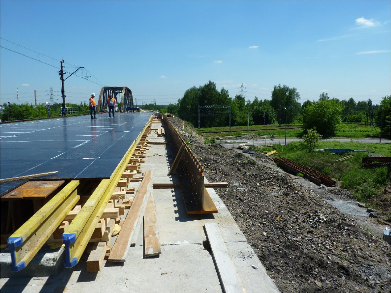
Figure 11
Steel T-sections on site next to scaffolding prepared for in situ slab (picture by Nowak Mosty).
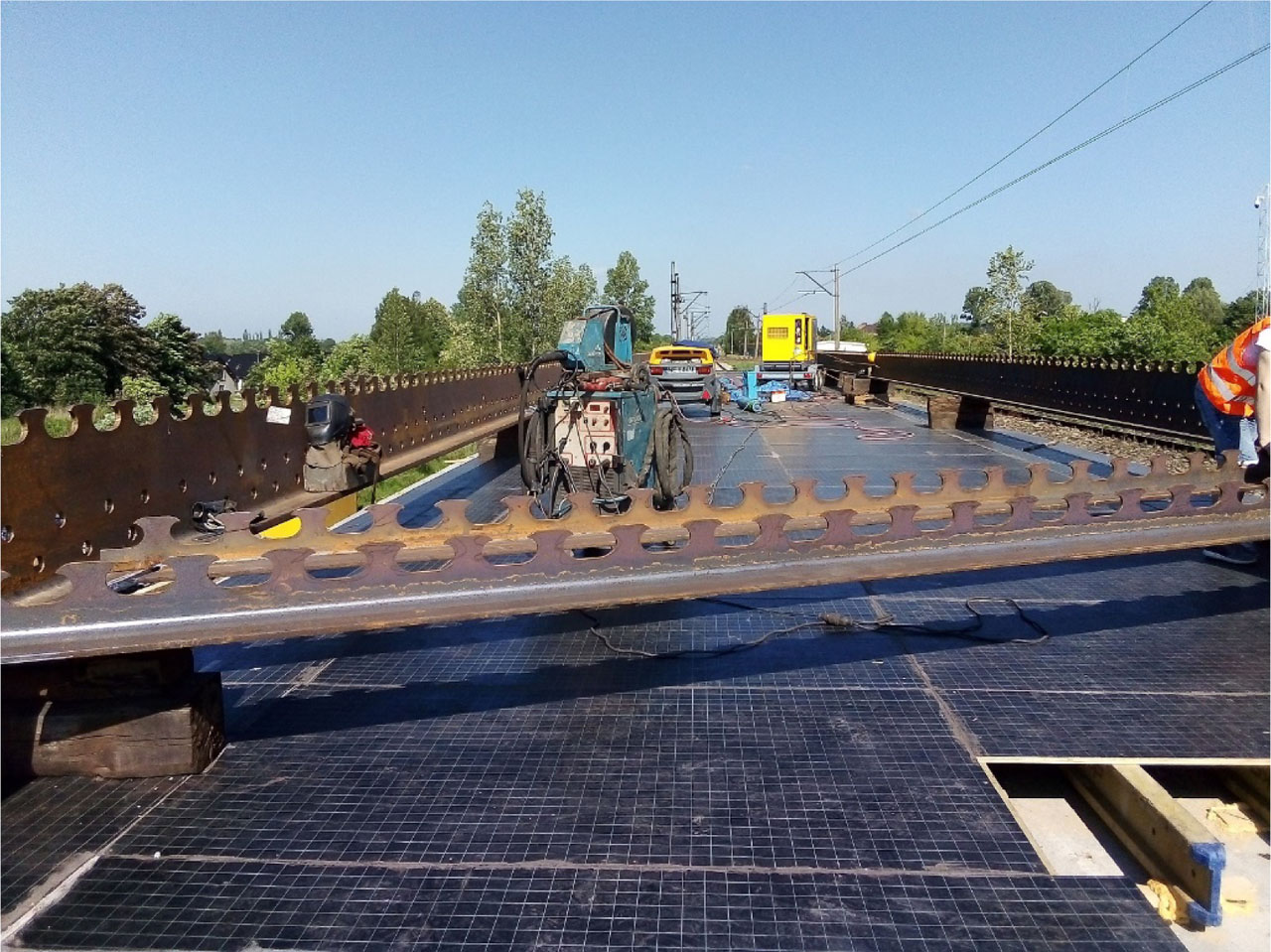
Figure 12
Steel structure after welding (picture by Nowak Mosty): main elements and transversal elements at the edge of slab.
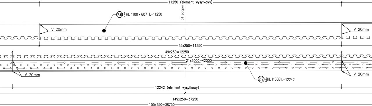
Figure 13
The geometry of the steel T-sections above the pillar [57].
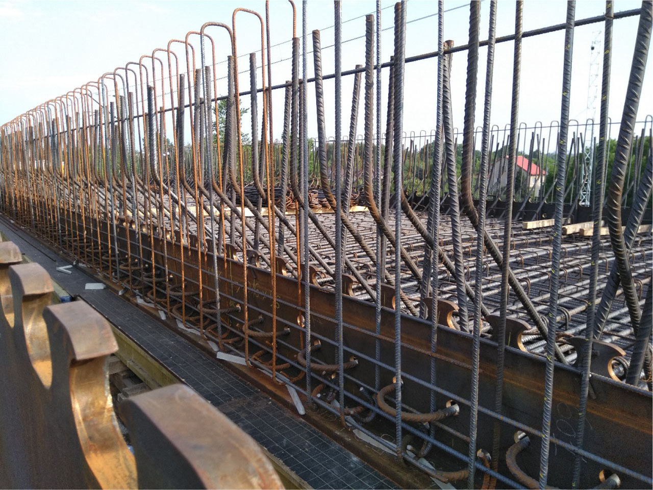
Figure 14
T-sections and reinforcement of bottom part of the superstructure (main stirrups crossing concrete dowels are still missing at this stage, compare Fig. 9).
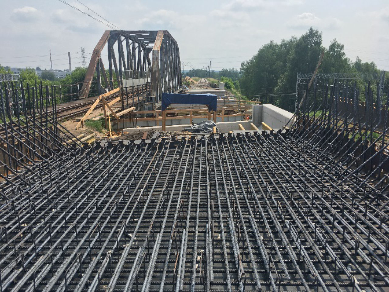
Figure 15
The general view of slab reinforcement.
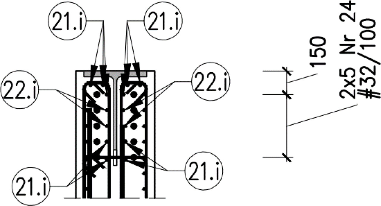
Figure 16
Reinforcing bars in the upper part of the web girders above the pillar [57].
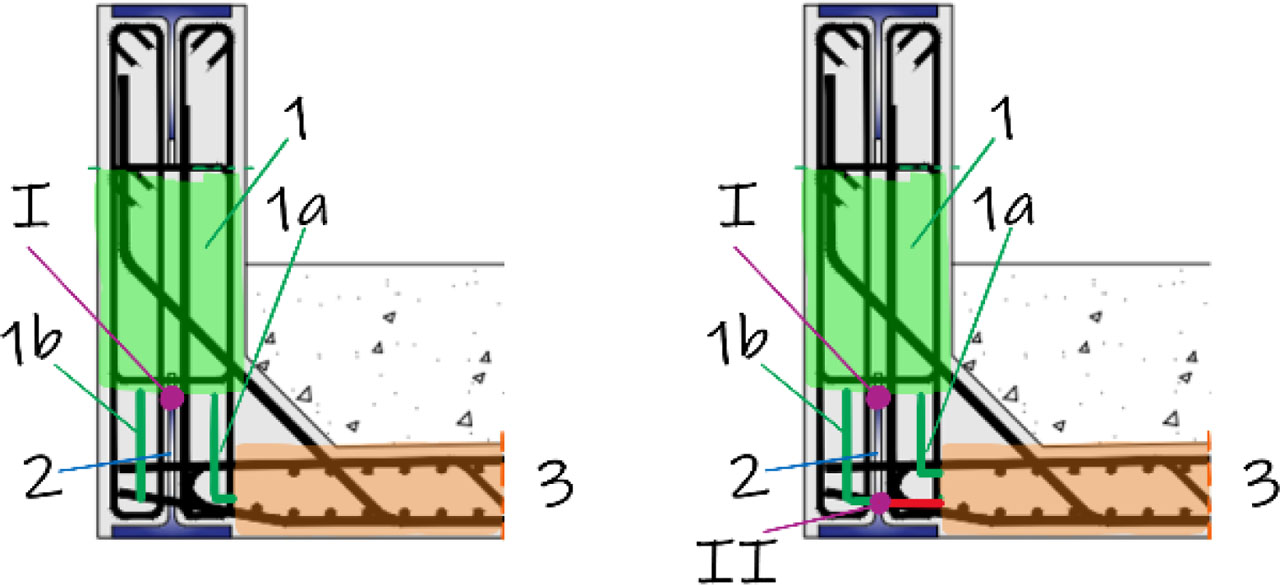
Figure 17
Possible longitudinal shear flow transfers: only via CDs (I) on the left and via CD (I) plus PBLs (II) on the right.
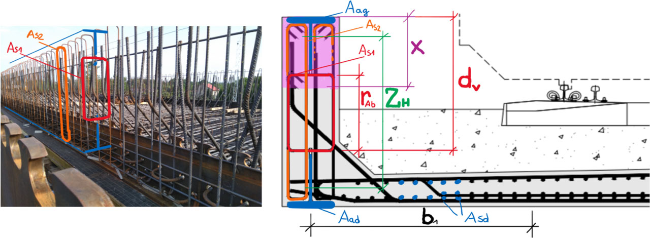
Figure 18
Implementation of the hybrid section concept (double composite) in the design of the bridge.
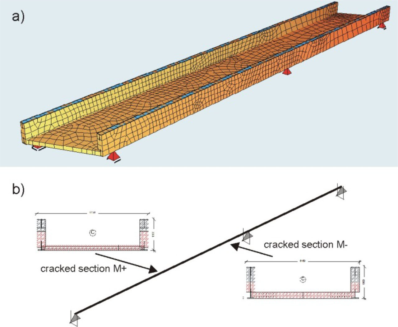
Figure 19
FEM models of the bridge structure made by external consulting [10]: a) mixed shell + beam model with shell elements standing for concrete parts and beam elements standing for structural steel parts; b) beam model using cracked steel–concrete sections.
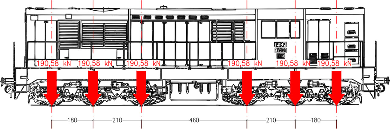
Figure 20
Scheme of the locomotive SM31.
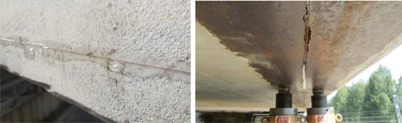
Figure 21
Optical fibers (light wires) on concrete and steel.
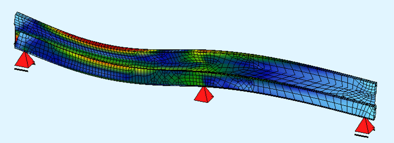
Figure 22
Exemplary deformation (linear analysis) of the finite element model from Fig. 19 under load 80 kN/m on the left span, applied as uniformly distributed to the slab in kPa [10].
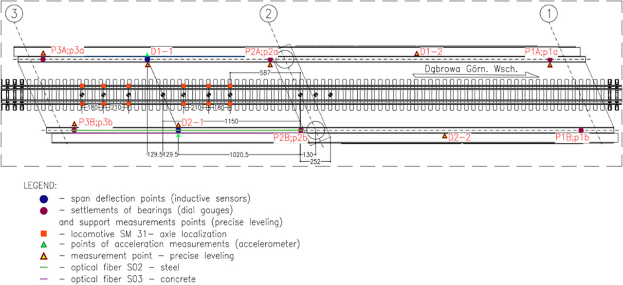
Figure 23
Load scheme and localization of measurements points.
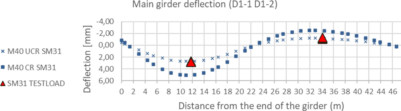
Figure 24
Main girder deflection of points no. D1-1 and D1-2 for models M40 CR and M40 UCR.
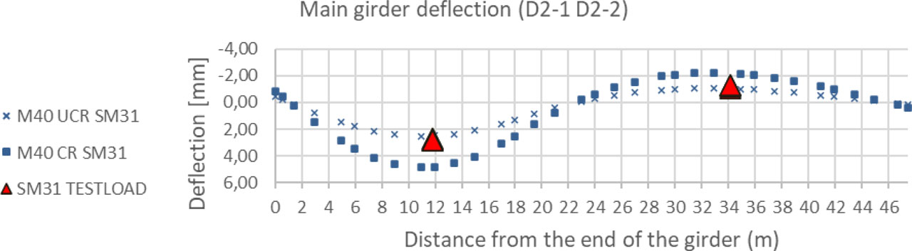
Figure 25
Main girder deflection of points no. D2-1 and D2-2 for models M40 CR and M40 UCR.
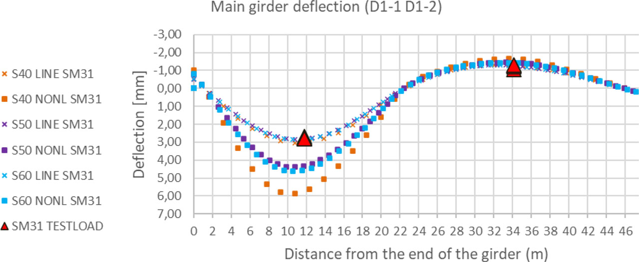
Figure 26
Main girder deflection of points no. D1-1 and D1-2 for models S40–S60 (LINE stands for linear, NONL stands for nonlinear material analysis).
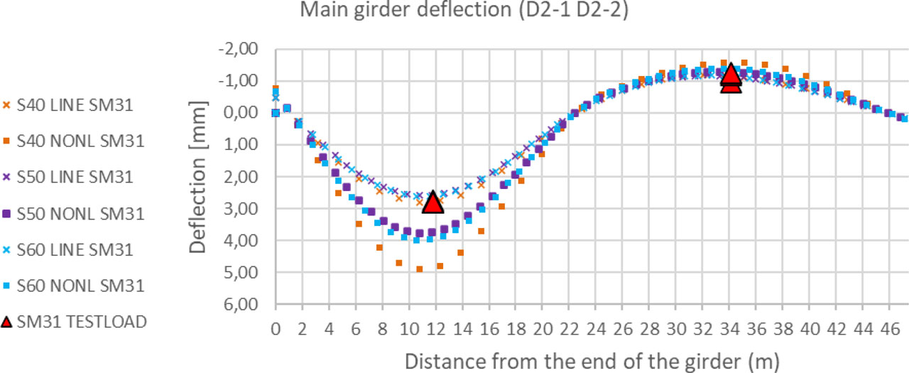
Figure 27
Main girder deflection of points no. D2-1 and D2-2 for models S40–S60.
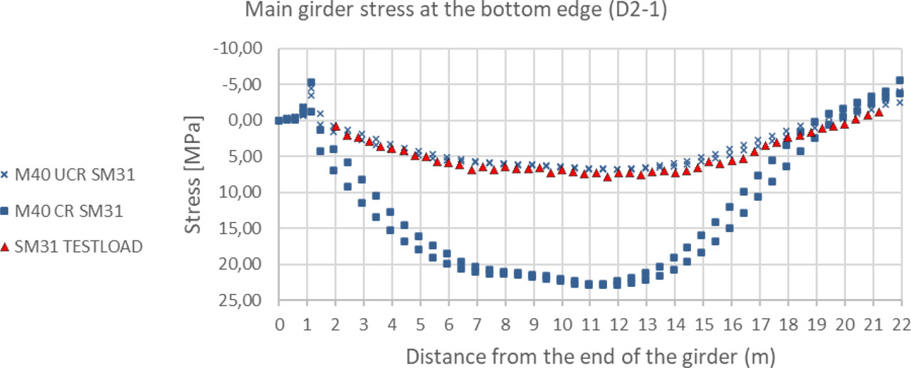
Figure 28
Stress in steel section for optical fibers and for the models M40 UCR/CR.
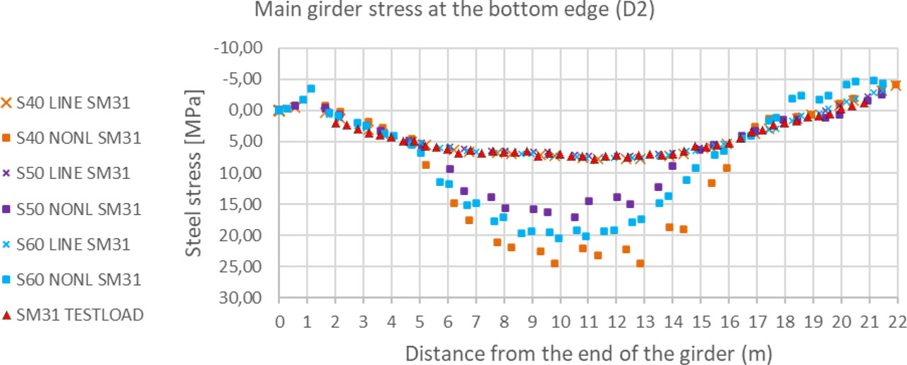
Figure 29
Stress in steel section for optical fibers and for the models S40–S60.
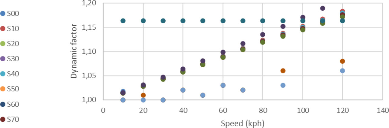
Figure 30
Comparison of dynamic factors for different FE models and the test load results.
Table 1
Dynamic factors for SOFiSTiK models.
| Speed | Dynamic factors | Units | |||||||||
|---|---|---|---|---|---|---|---|---|---|---|---|
| Model no. | - | S00 | S10 | S20 | S30 | S40 | S50 | S60 | S70 | - | |
| Maintenance | - | Standard | - | ||||||||
| Span length | LΦ | 26.85 | m | ||||||||
| Frequency | n0 | 4.83 | 4.45 | 4.68 | 4.70 | 4.57 | 4.83 | 4.72 | 4.71 | Hz | |
| ϕ | 10 | 2.78 | 1.02 | 1.01 | 1.01 | 1.01 | 1.01 | 1.01 | 1.01 | 1.01 | - |
| 20 | 5.56 | 1.03 | 1.03 | 1.03 | 1.03 | 1.03 | 1.03 | 1.03 | 1.03 | ||
| 30 | 8.33 | 1.04 | 1.04 | 1.04 | 1.04 | 1.04 | 1.04 | 1.04 | 1.04 | ||
| 40 | 11.11 | 1.06 | 1.06 | 1.06 | 1.06 | 1.06 | 1.06 | 1.06 | 1.06 | ||
| 50 | 13.89 | 1.07 | 1.07 | 1.07 | 1.07 | 1.07 | 1.07 | 1.07 | 1.07 | ||
| 60 | 16.67 | 1.09 | 1.09 | 1.09 | 1.09 | 1.09 | 1.09 | 1.09 | 1.09 | ||
| 70 | 19.44 | 1.10 | 1.11 | 1.10 | 1.10 | 1.11 | 1.10 | 1.10 | 1.10 | ||
| 80 | 22.22 | 1.12 | 1.12 | 1.12 | 1.12 | 1.12 | 1.12 | 1.12 | 1.12 | ||
| 90 | 25.00 | 1.13 | 1.14 | 1.13 | 1.13 | 1.14 | 1.13 | 1.13 | 1.13 | ||
| 100 | 27.78 | 1.15 | 1.15 | 1.15 | 1.15 | 1.15 | 1.15 | 1.15 | 1.15 | ||
| 110 | 30.56 | 1.16 | 1.17 | 1.16 | 1.16 | 1.16 | 1.16 | 1.16 | 1.16 | ||
| 120 | 33.33 | 1.17 | 1.18 | 1.18 | 1.18 | 1.18 | 1.17 | 1.18 | 1.18 | ||
| Speed | Dynamic factors | Units | |||||||||
Table 2
Dynamic factors for Midas models, PN-EN 1991-2, and test values.
| Speed | Dynamic factors | Units | ||||||
|---|---|---|---|---|---|---|---|---|
| Model no. | - | M40 UCR | M40 CR | 6.4.5.2 | D1 | D2 | - | |
| Maintenance | - | Standard | - | - | - | |||
| Span length | LΦ | 26.85 | - | - | m | |||
| Frequency | n0 | 4.90 | 3.76 | - | 5.43 | Hz | ||
| ϕ | 10 | 1.01 | 1.02 | 1.16 | 1.00 | 1.00 | - | |
| 20 | 1.03 | 1.03 | 1.16 | 1.01 | 1.00 | |||
| 30 | 1.04 | 1.05 | 1.16 | 1.00 | 1.00 | |||
| 40 | 1.06 | 1.06 | 1.16 | 1.02 | 1.02 | |||
| 50 | 1.07 | 1.08 | 1.16 | 1.01 | 1.01 | |||
| 60 | 1.09 | 1.10 | 1.16 | 1.03 | 1.03 | |||
| 70 | 1.10 | 1.12 | 1.16 | 1.02 | 1.02 | |||
| 80 | 1.12 | 1.13 | 1.16 | - | - | |||
| 90 | 1.13 | 1.15 | 1.16 | 1.06 | 1.03 | |||
| 100 | 1.14 | 1.17 | 1.16 | - | - | |||
| 110 | 1.16 | 1.19 | 1.16 | - | - | |||
| 120 | 1.17 | 1.21 | 1.16 | 1.08 | 1.06 | |||
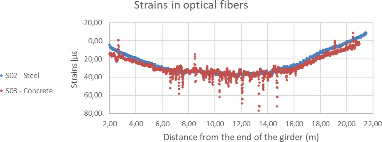
Figure 31
Strain in optical fibers along the span.
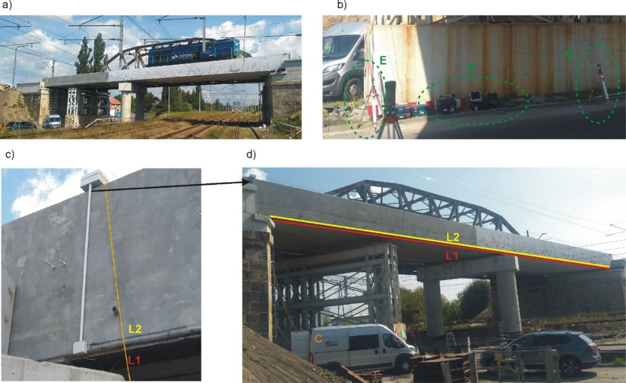
Figure 32
General view of the structure during test. L1 – light wire on steel flange, L2 – light wire on concrete web, E – measuring equipment under the bridge (displacements), C – car with computer for computing light wire recordings.