
Table 1
Designation and details of type of soil in upper and lower layers under both types of footings in two-layered soils.
| Designation | Soil type in upper and lower layers for two-layered soil | |
|---|---|---|
| Case 1 | Upper layer | Unstabilized clay |
| Lower layer | Medium-dense sand | |
| Case 2 | Upper layer | Stabilized clay (C:M:: 90:10) |
| Lower layer | Medium-dense sand | |
| Case 3 | Upper layer | Stabilized clay (C:WFS:: 80:20) |
| Lower layer | Medium-dense sand | |
| Case 4 | Upper layer | Stabilized clay (C: L:: 91:9) |
| Lower layer | Medium-dense sand | |
| Case 5 | Upper layer | Stabilized clay (C:M:WFS:: 80:10:10) |
| Lower layer | Medium-dense sand | |
| Case 6 | Upper layer | Stabilized clay (C:M:L:: 84:10:6) |
| Lower layer | Medium-dense sand | |
| Case 7 | Upper layer | Stabilized clay (C:WFS:L:: 74:20:6) |
| Lower layer | Medium-dense sand | |
| Case 8 | Upper layer | Stabilized clay (C:M:WFS:L:: 67:10:20:3) |
| Lower layer | Medium-dense sand | |
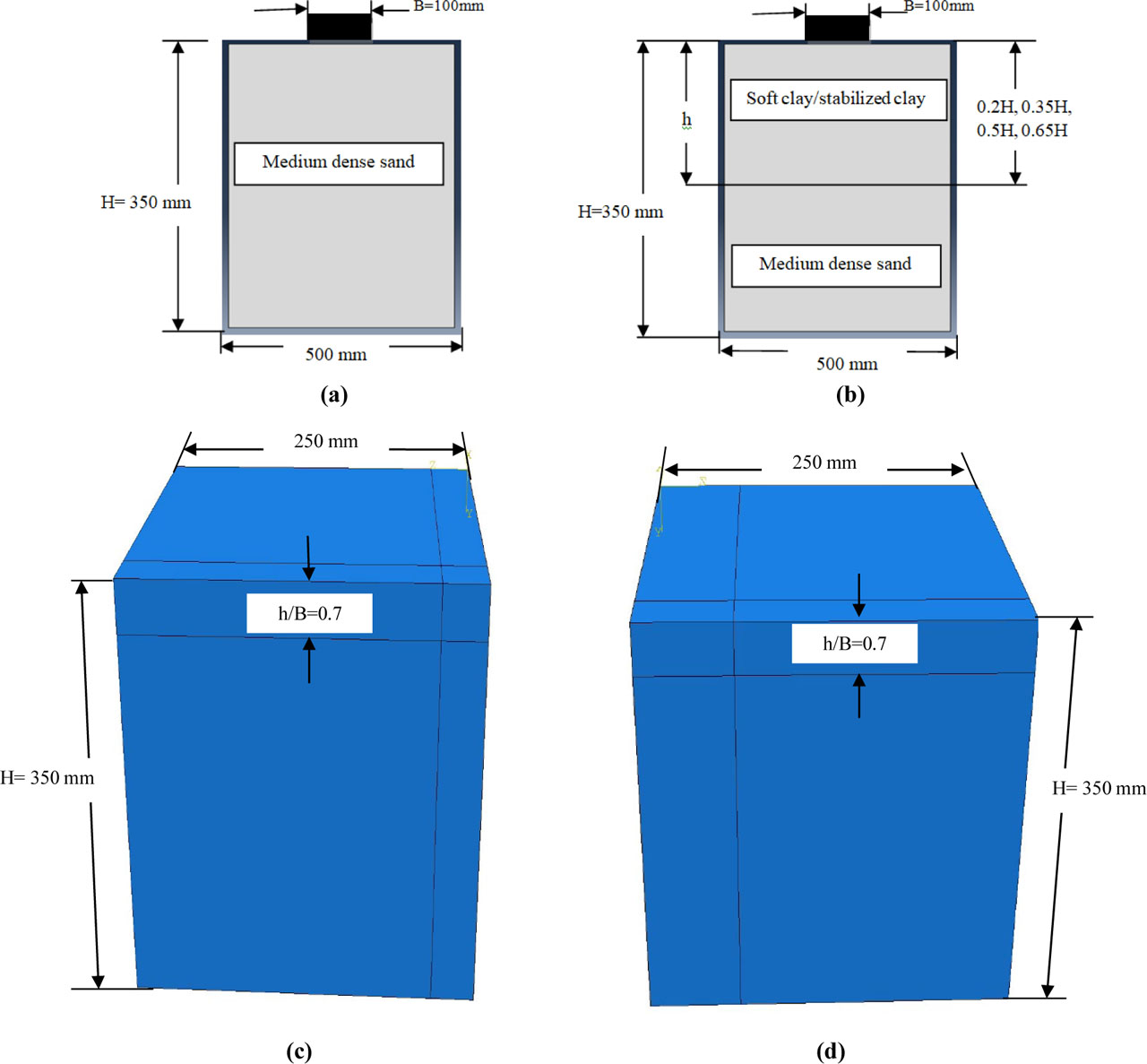
Figure 1
Problem definition. (a) Single layer; (b) thickness of top layer varying at h/B=0.7, 1.225, 1.75, and 2.275; (c) FEM model of footing for aspect ratio (L/B) =1 at h/B=0.7; (d) FEM model of footing for aspect ratio (L/B) =2 at h/B=0.7. h: thickness of the upper layer in two-layered soil; L, B:length and width of footing, respectively
Note: all dimensions are not to scale.
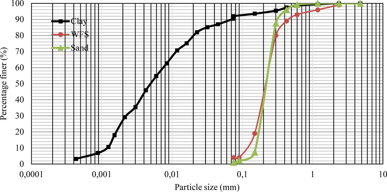
Figure 2
Particle size curve for clayey soil and WFS.
Table 2
Geotechnical properties of clayey soil.
| Soil properties | Value |
|---|---|
| Soil type | CH |
| Liquid limit | 55% |
| Plastic limit | 20% |
| Plasticity index | 35% |
| Specific gravity | 2.6 |
| Differential free swell index | 35% |
| Optimum moisture content | 16.5% |
Table 3
Mineral composition of clayey soil.
| Mineral composition | Content (%) |
|---|---|
| Oxygen, O | 45.4 |
| Silicon, Si | 18.5 |
| Aluminum, Al | 8.69 |
| Carbon, C | 10.9 |
| Iron, Fe | 1.42 |
| Potassium, K | 1.86 |
| Magnesium, Mg | 2.30 |
| Titanium, Ti | 2.51 |
Table 4
Chemical properties of molasses used.
| Constituents | Result |
|---|---|
| Color | Black |
| Brix | 83.2 |
| pH (1:1 at 20°C) | 5.6 |
| Specific gravity | 1.39 |
| Viscosity | 17,500 mPas |
| Moisture | 21.76% |
| Total sugar | 47.83% |
| Invert sugar | 10.20% |
| Sulfated sugar | 15.50% |
| Ca | 1.63% |
Table 5
Geotechnical properties of WFS.
| Property | Value |
|---|---|
| Specific gravity | 2.64 |
| Optimum moisture content | 8.20% |
| Maximum dry density | 1.59 g/cc |
Table 6
Chemical properties of WFS.
| Chemical composition | Percentage |
|---|---|
| SiO2 | 84.90 |
| Al2O3 | 5.21 |
| Fe2O3 | 3.32 |
| CaO | 0.58 |
| MgO | 0.67 |
| SO3 | 0.29 |
| MnO | 0.08 |
| TiO2 | 0.19 |
| K2O | 0.97 |
| P2O5 | 0.05 |
| Na2O | 0.50 |
| ¬Loss of ignition | 2.87 |
Table 7
Chemical composition of lime used.
| Chemical composition | Content (%) |
|---|---|
| SiO2 | 2.1 |
| Al2O3 | 1.3 |
| Fe2O3 | 1.2 |
| CaO | 82.8 |
| MgO | 0.3 |
| SO3 | 0.4 |
| Na2O | 0.4 |
| K2O | - |
| TiO2 | - |
| C | 2.2 |
| CaCO3 | 4.3 |
| Impurities | 5.0 |
| ¬Loss of ignition at 800°C | - |
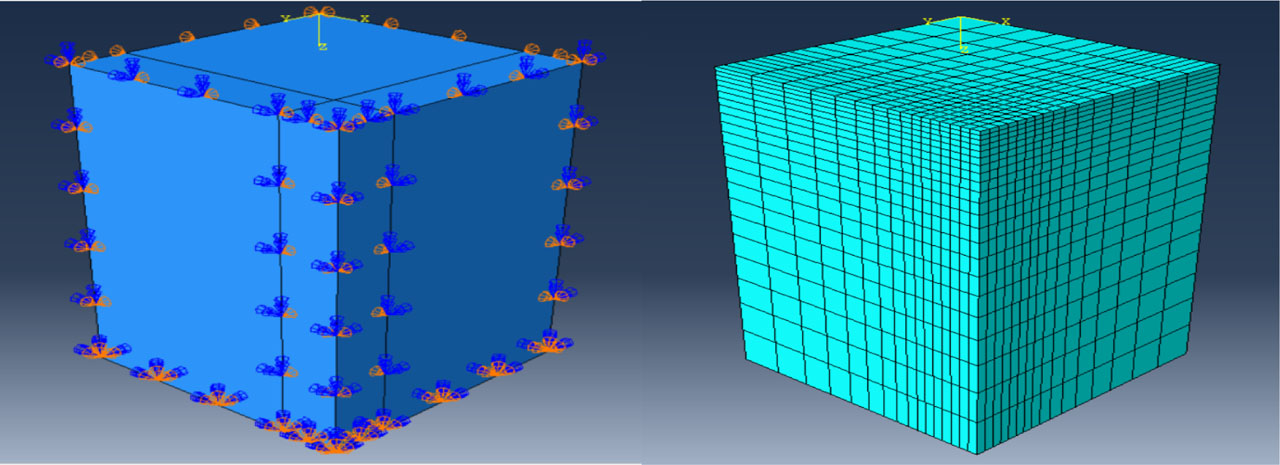
Figure 3
Finite element discretization and boundary condition selection of the footing model with L/B=1.
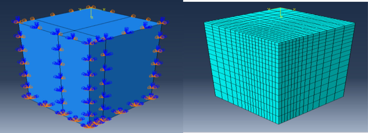
Figure 4
Finite element discretization and boundary condition selection of the footing model with L/B=2.
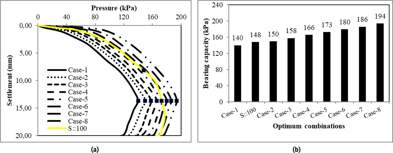
Figure 5
(a) Pressure–settlement curves and (b) bearing capacity values of two-layered soil for all cases at h/B=0.7 and single-layer sandy soil for L/B=1.
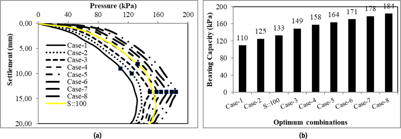
Figure 6
(a) Pressure–settlement curves and (b) bearing capacity values of two-layered soil for all cases at h/B=0.7 and single-layer sandy soil for L/B=2.
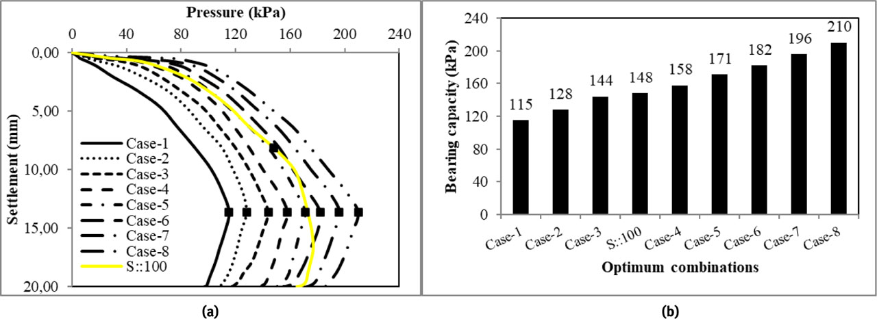
Figure 7
(a) Pressure–settlement curves and (b) bearing capacity values of two-layered soil for all cases at h/B=1.225 and single-layer sandy soil for L/B=1.
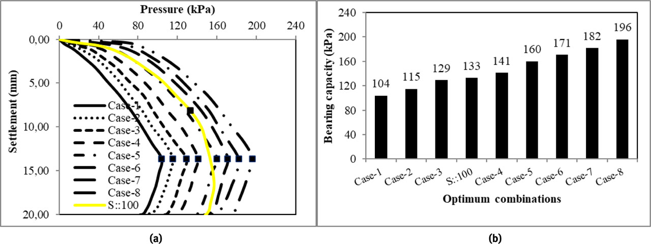
Figure 8
(a) Pressure–settlement curves and (b)) bearing capacity values of two-layered soil for all cases at h/B=1.225 and single-layer sandy soil for L/B=2
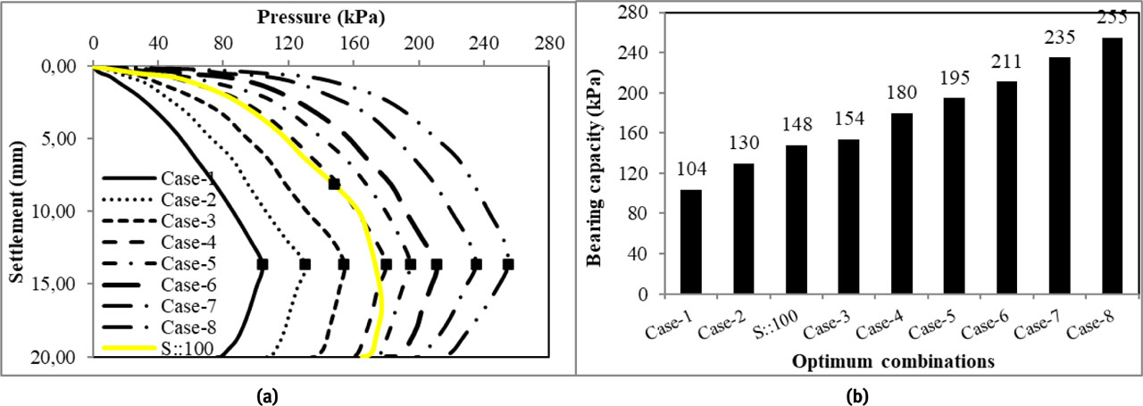
Figure 9
(a) Pressure–settlement curves and (b) bearing capacity values of two-layered soil for all cases at h/B=1.75 and of single-layer sandy soil for L/B=1.
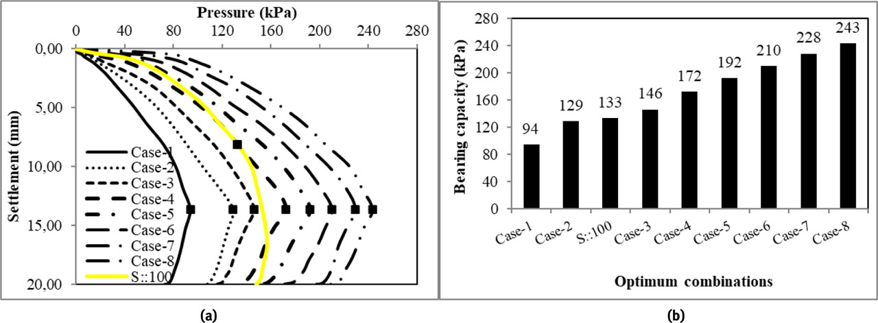
Figure 10
(a) Pressure–settlement curves and (b) bearing capacity values of two-layered soil for all cases at h/B=1.75 and of single-layer sandy soil for L/B=2.
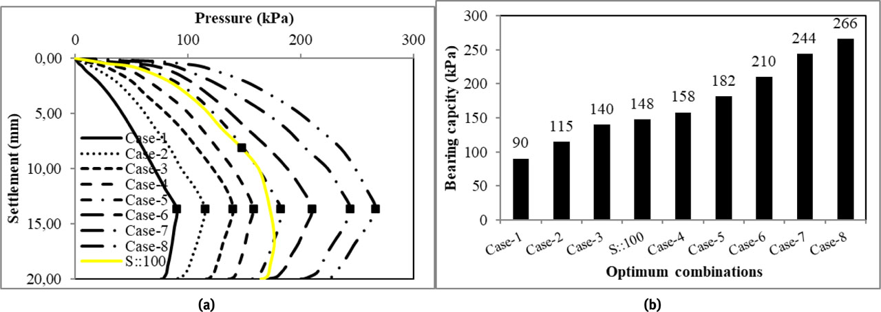
Figure 11
(a) Pressure–settlement curves and (b) bearing capacity values of two-layered soil for all cases at h/B=2.275 and single-layer sandy soil for L/B=1.
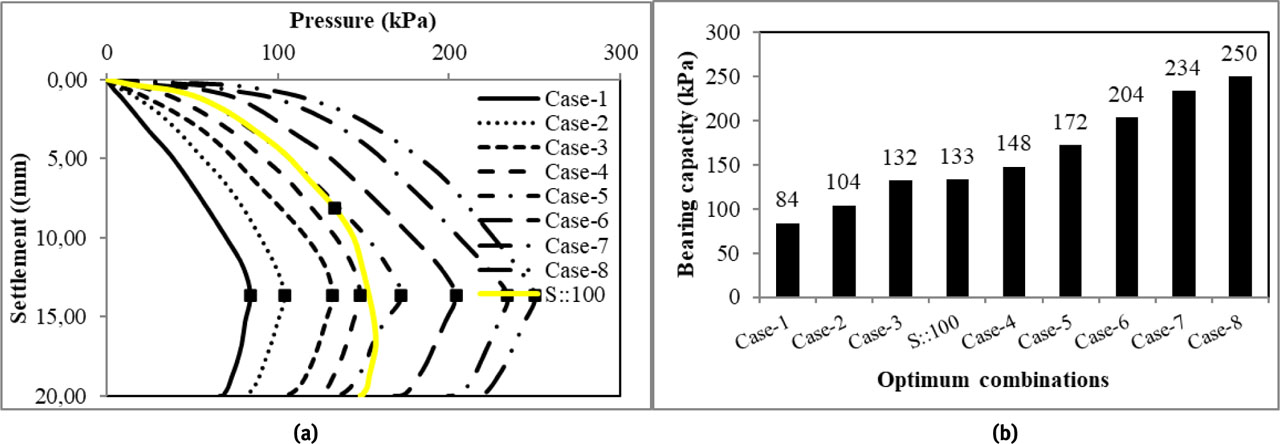
Figure 12
(a) Pressure–settlement curves and (b) bearing capacity values of two-layered soil for all cases at h/B=2.275 and single-layer sandy soil for L/B=2.
Table 8
Material properties of unstabilized/stabilized clayey soil and sandy soil (Mohr–Coulomb model) [23].
| C | C:M | C:WFS | C:L | C:M:WFS | C:M:L | C:WFS:L | C:M:WFS:L | S::100 | |
|---|---|---|---|---|---|---|---|---|---|
| Mass density (γ) (kg/m3) | 1710 | 1790 | 1781 | 1606 | 1840 | 1750 | 1730 | 1820 | 1615 |
| Modulus of elasticity (E) (MPa) | 3.2 | 5.3 | 7.2 | 9.6 | 10.3 | 14.7 | 16.2 | 18.5 | 32.3 |
| Poisson ratio (ν) | 0.3 | 0.3 | 0.3 | 0.32 | 0.33 | 0.34 | 0.36 | 0.38 | 0.3 |
| Angle of internal friction (ϕ) | 14.86 | 17.06 | 19.11 | 21.43 | 23.62 | 25.64 | 27.85 | 29.68 | 35 |
| Cohesion (c) (kPa) | 21.77 | 19.92 | 19.08 | 17.61 | 16.43 | 15.59 | 14.78 | 13.89 | 0.1 |
Table 9
Comparison of observed bearing capacity values with Vesic (1973), Hansen (1970), and Terzaghi (1943) calculations.
| Present study | Vesic (1973) | Hansen (1970) | Terzaghi (1943) | |||||
|---|---|---|---|---|---|---|---|---|
| Sand | L/B=1 | L/B=2 | L/B=1 | L/B=2 | L/B=1 | L/B=2 | L/B=1 | L/B=2 |
| 148 | 133 | 138 | 121.78 | 113.27 | 106.11 | 94.25 | 97.67 | |
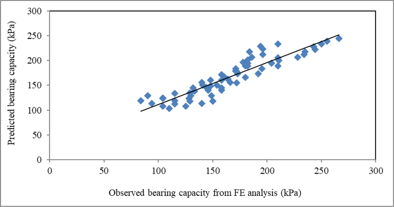
Figure 13
Variation of numerical and predicted bearing capacity for both footings (L/B= 1, 2).
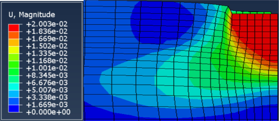
Figure 14
Displacement contours of case 1 at h/B = 0.7 for L/B=1.
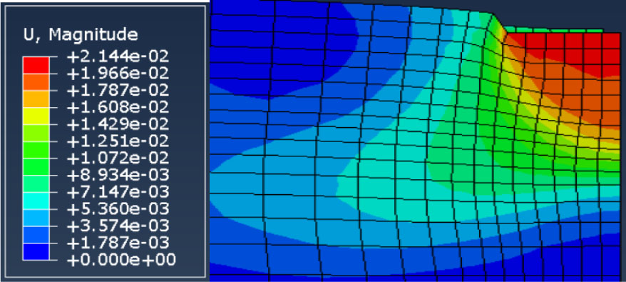
Figure 15
Displacement contours of case 8 at h/B = 0.7 for L/B=1.
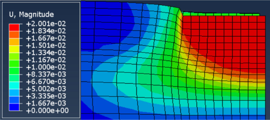
Figure 16
Displacement contours of case 1 at h/B = 0.7 for L/B=2.
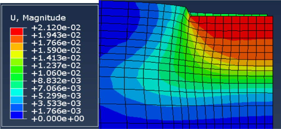
Figure 17
Displacement contours of case 8 at h/B = 0.7 for L/B=2.
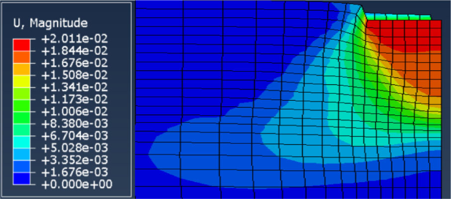
Figure 18
Displacement contours of case 1 at h/B = 1.225 for L/B=1.
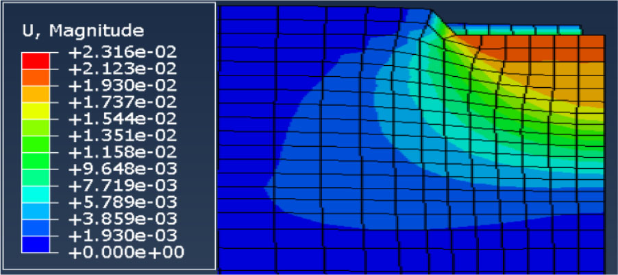
Figure 19
Displacement contours of case 8 at h/B = 1.225 for L/B=1.
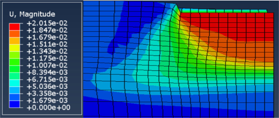
Figure 20
Displacement contours of case 1 at h/B = 1.225 for L/B=2.
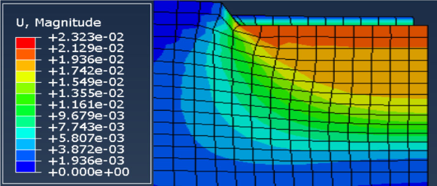
Figure 21
Displacement contours of case 8 at h/B = 1.225 for L/B=2.
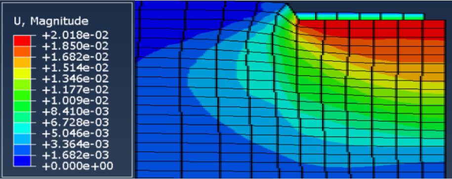
Figure 22
Displacement contours of case 1 at h/B = 1.75 for L/B=1.
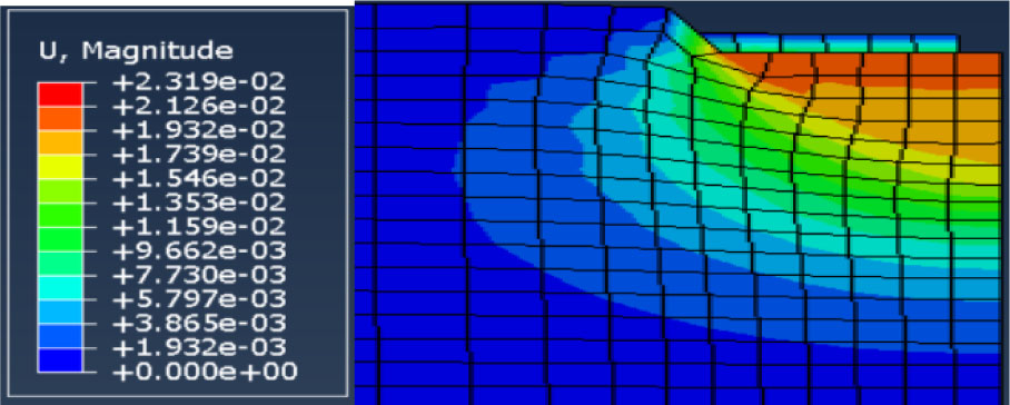
Figure 23
Displacement contours of case 8 at h/B = 1.75 for L/B=1
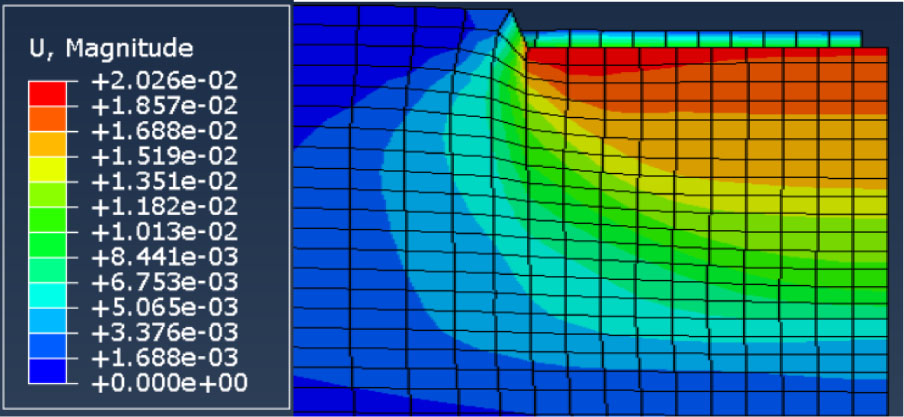
Figure 24
Displacement contours of case 1 at h/B = 1.75 for L/B=2.
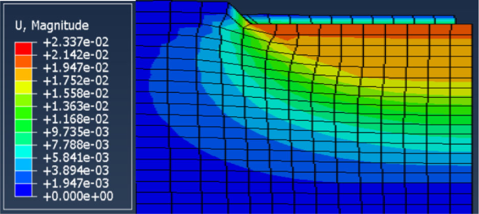
Figure 25
Displacement contours of case 8 at h/B = 1.75 for L/B=2
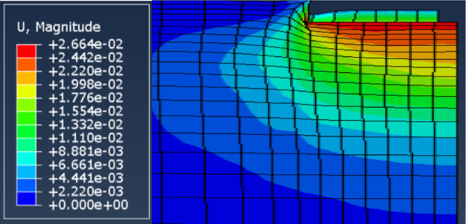
Figure 26
Displacement contours of case 1 at h/B = 2.275 for L/B=1.
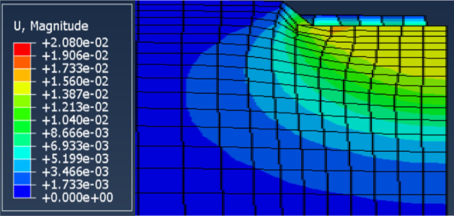
Figure 27
Displacement contours of case 8 at h/B = 2.275 for L/B=1.
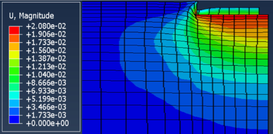
Figure 28
Displacement contours of case 1 at h/B = 2.275 for L/B=2.
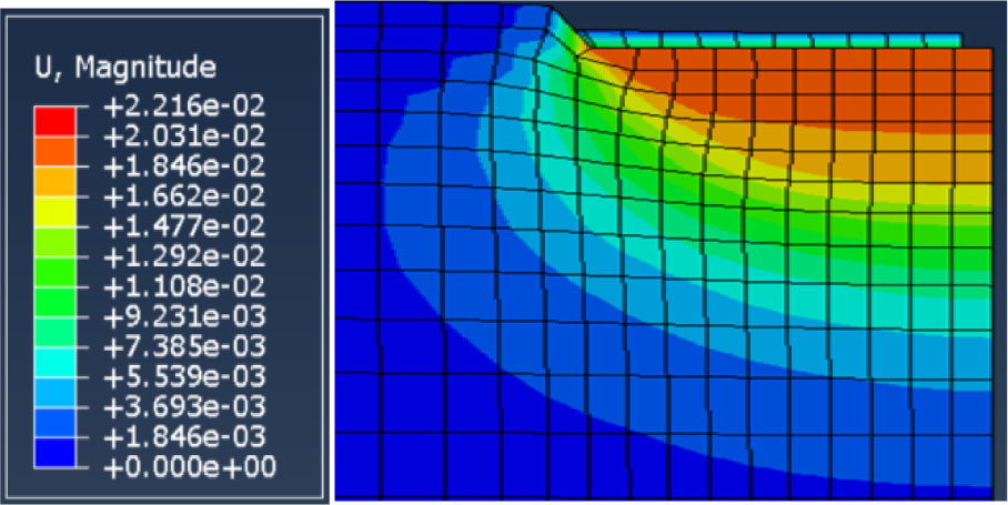
Figure 29
Displacement contours of case 8 at h/B = 2.275 for L/B=2.