
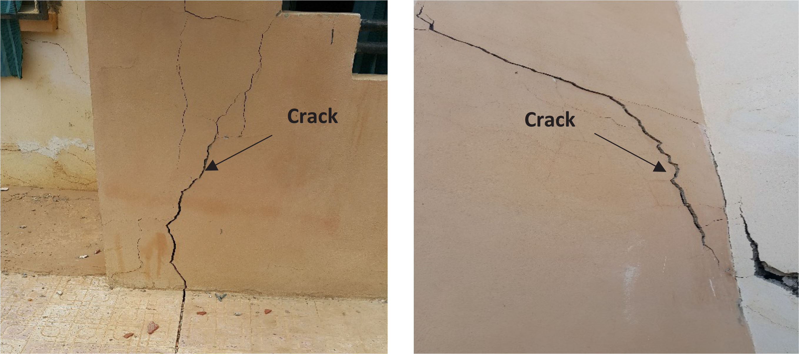
Figure 1
Example of damage of swelling soil in N’Gaous city.
Table 1
Geotechnical characteristics of soil samples.
| Soil properties | Value |
|---|---|
| Sampling depth | 2.3–2.5 m |
| Liquid limit, LL (%) | 72.28 |
| Plastic limit, PL (%) | 29.20 |
| Plasticity Index, PI (%) | 43.08 |
| Natural dry unit weight, γd (kN/m3) | 17.5 |
| Natural wet unit weight, γh (kN/m3) | 20.0 |
| Specific Gravity, Gs | 2.74 |
| Natural water content, Wn (%) | 14.1 |
| Natural degree of saturation, Sr (%) | 80.82 |
| Initial void ratio, e0 | 0.478 |
| Compression Index, Cc | 0.15 |
| Swelling Index, Cs | 0.054 |
| Preconsolidation pressure, Pc (kPa) | 190 |
| Cohesion, after saturation C (kPa) | 100 |
| Friction angle, after saturation φ (°) | 25 |
| Grain size distribution | 71 |
| Clay (%) | 24.5 |
| Silt (%) | 4.5 |
| Sand (%) | 98.90 |
| C80 μm (%) | 71 |
| C2 μm (%) |
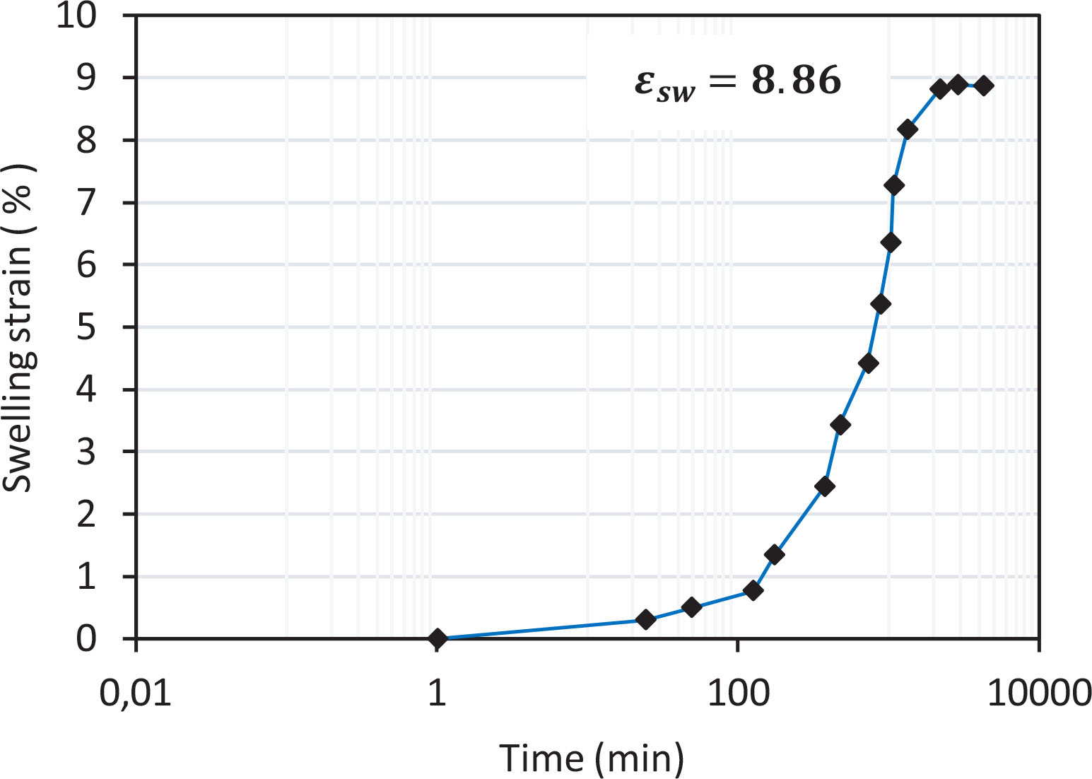
Figure 2
Free swelling strain versus elapsed time.
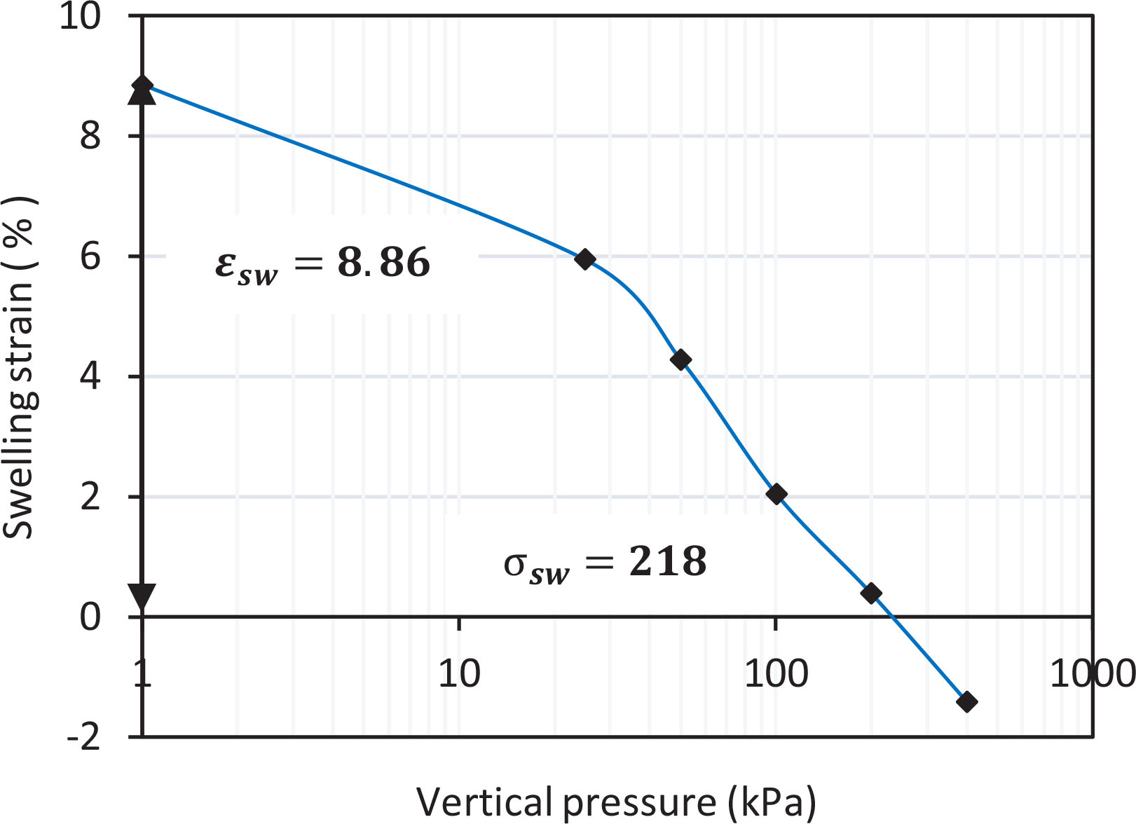
Figure 3
Swelling strain versus vertical pressure
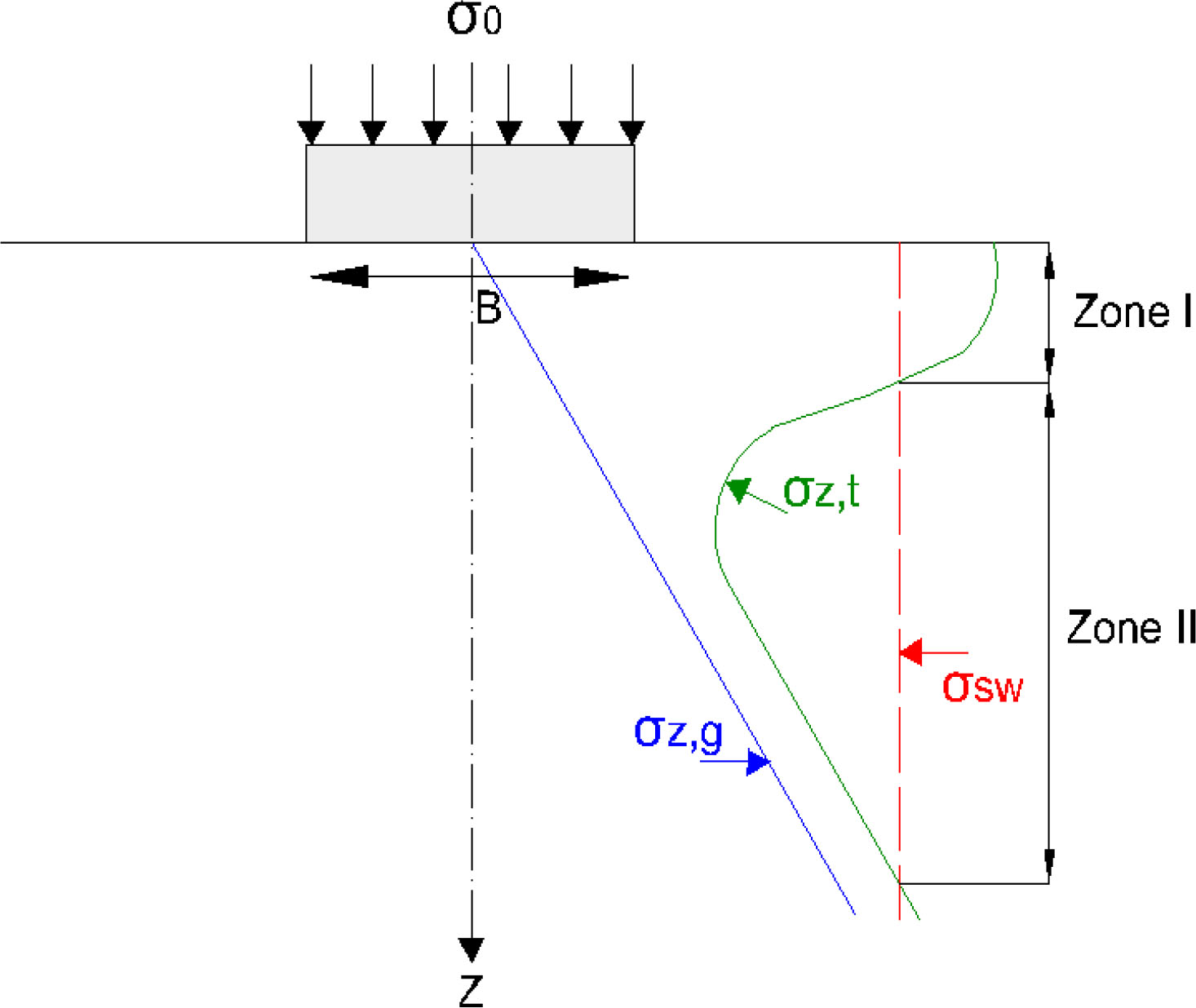
Figure 4
Scheme of stresses distributions in the soil below a shallow foundation.
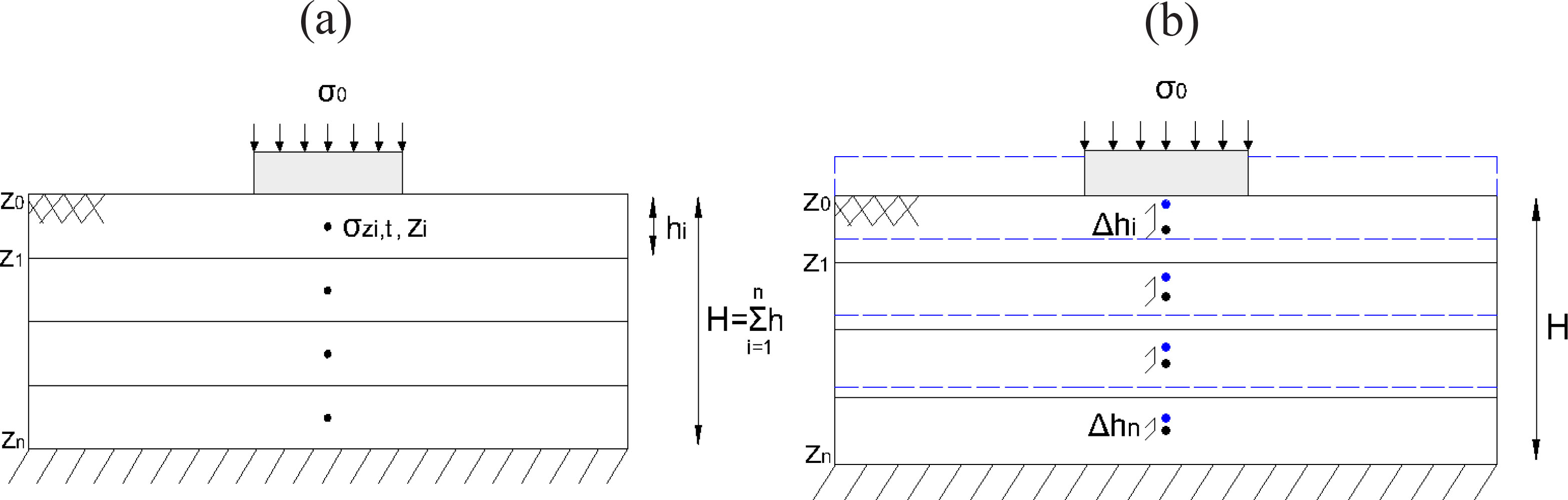
Figure 5
(a) Initial states of layers, (b) Final states of layers after total heave.
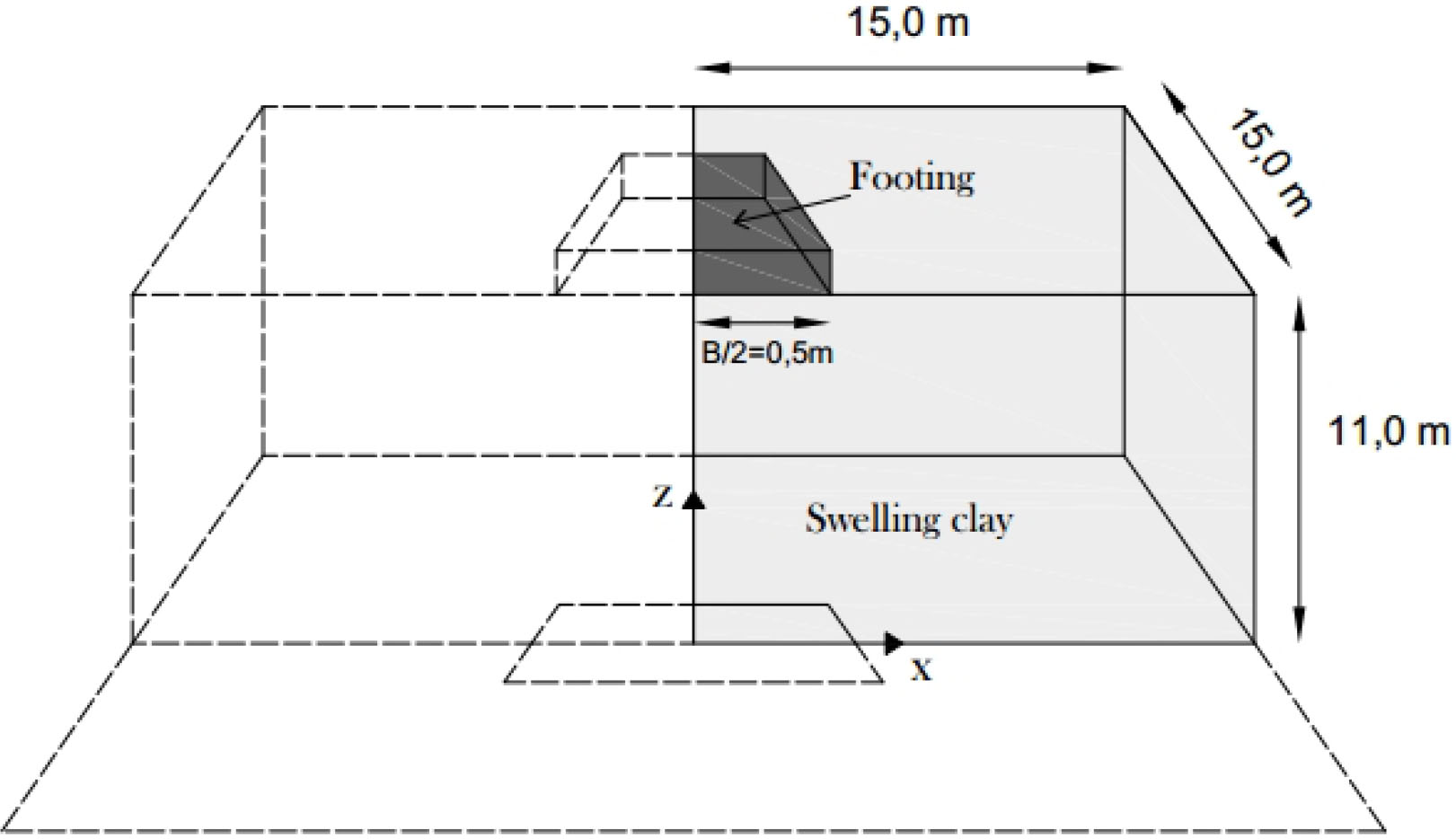
Figure 6
Geometry of the model.
Table 2
Soils parameters used in the numerical study.
| Parameters | Value |
|---|---|
| Unit weight, γ (kN/m3) | 20 |
| Elastic Modulus, E (MPa) | 10 |
| Poisson's ratio, ν | 0.35 |
| Cohesion, C (kPa) | 100 |
| Friction angle, φ (°) | 25 |
| Dilatancy angle, ψ (°) | 0 |
[i] Note: ;
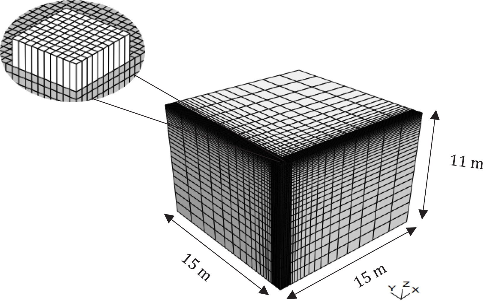
Figure 7
Three-dimensional mesh of the numerical model.
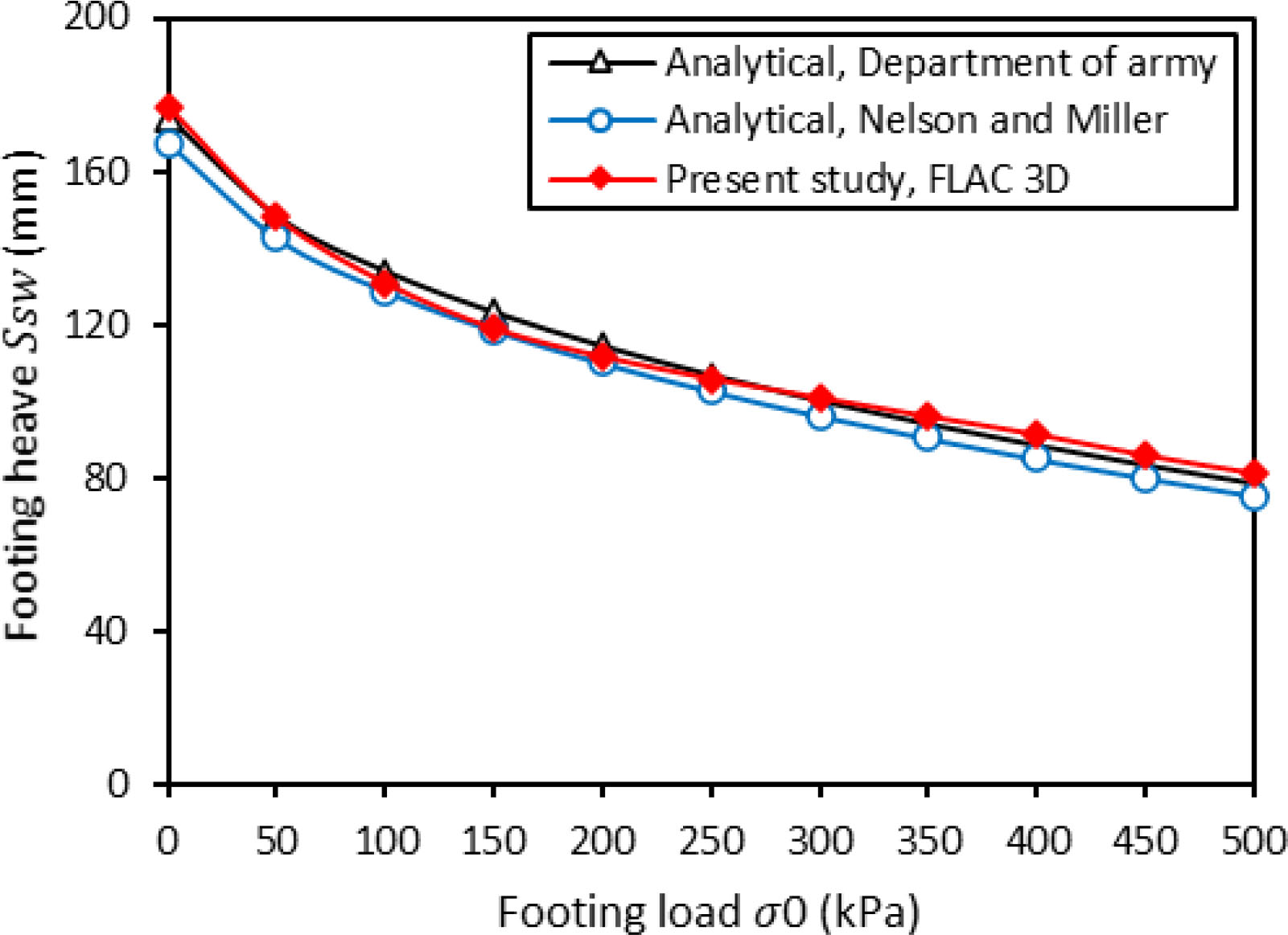
Figure 8
Comparison of heave results Ssw for square footing obtained from numerical and analytical prediction.
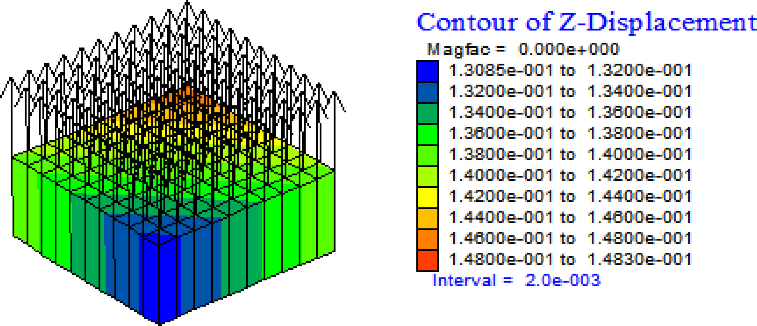
Figure 9
Contours and vectors heaving of square footing for σ0=100 kPa.
Table 3
Heave prediction for each type of isolated shallow foundations from numerical and analytical analysis.
| Foundation Type | Foundation Heave Ssw (mm) | Applied Loads σ0(kPa) | |||||
|---|---|---|---|---|---|---|---|
| 0 | 100 | 200 | 300 | 400 | 500 | ||
| Rectangle B = 1 m, L = 2 m | Calculated | ||||||
| Nelson and Miller | 167.5 | 121.3 | 98.9 | 82.42 | 68.99 | 57.48 | |
| Department of army | 173.7 | 125.79 | 102.56 | 85.47 | 71.54 | 59.61 | |
| Numerical | 158 | 125.2 | 108.9 | 96.1 | 83.7 | 71.2 | |
| Circle D = 1.8 m | Calculated | ||||||
| Nelson and Miller | 167.5 | 130.6 | 110.9 | 96.2 | 84.1 | 73.6 | |
| Department of army | 173.7 | 135.48 | 115.08 | 99.8 | 87.22 | 76.39 | |
| Numerical | 157.2 | 125.1 | 108.6 | 94.5 | 80.5 | 66.3 | |
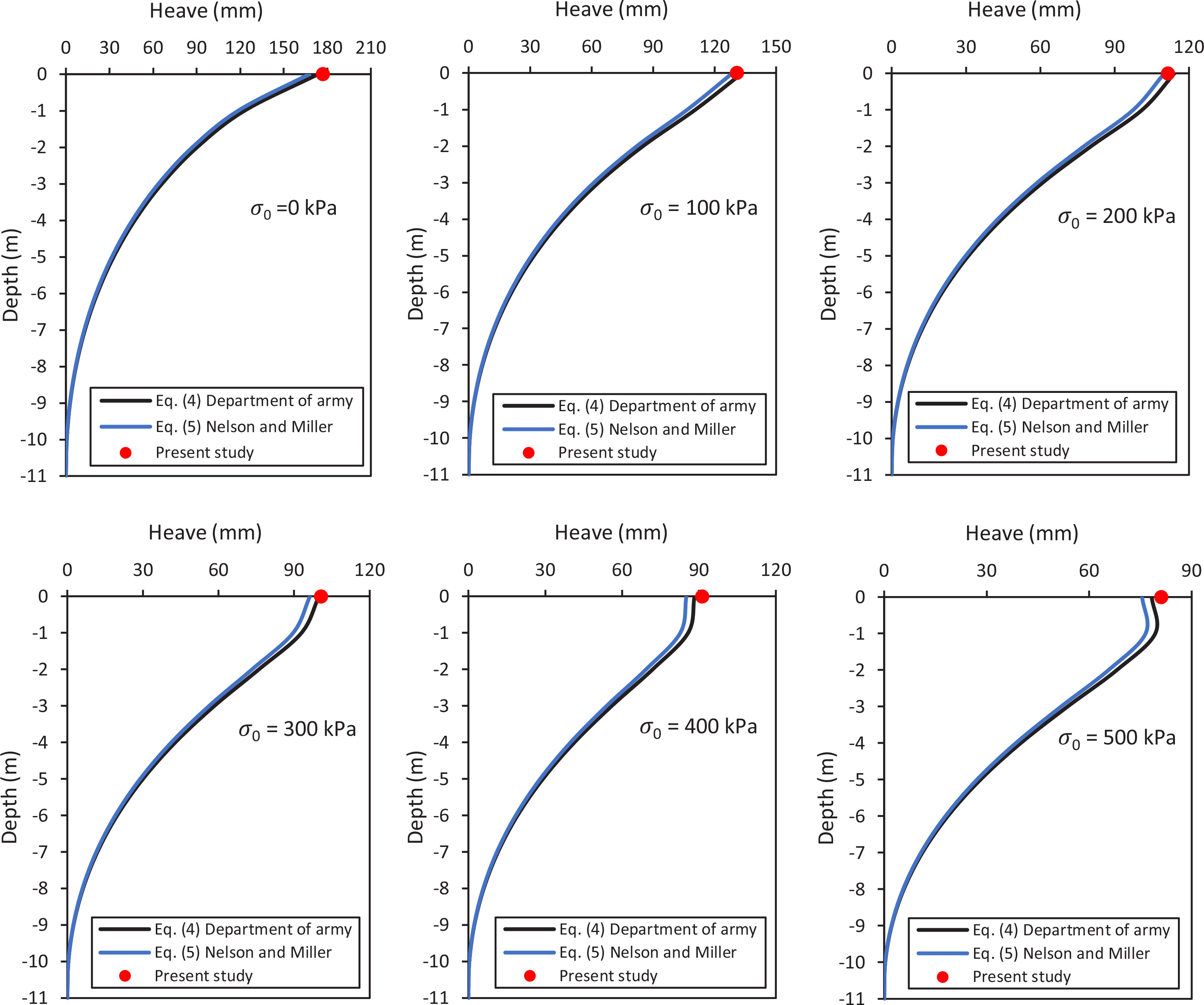
Figure 10
Comparison between numerical and analytical results of heave evolutions throughout the soil depth. Case of square footing of width B=1m and σ0=0 to 500 kPa.
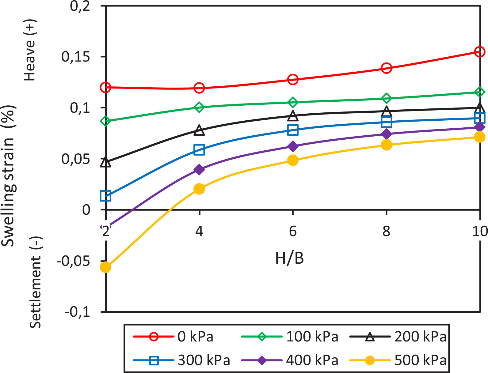
Figure 11
Variation of vertical swelling strain ɛsw after swelling for square footing with H/B ratio and σ0=0 to 500 kPa.
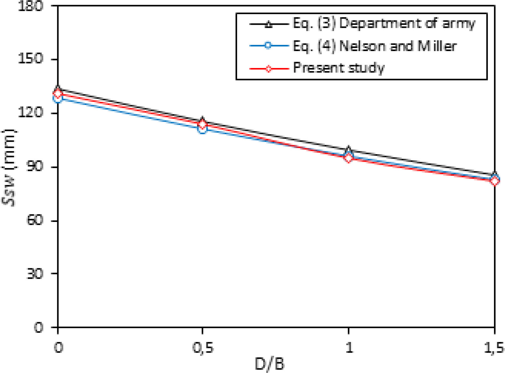
Figure 12
Comparison between numerical and analytical results of square footing heave Ssw with D/B ratio for σ0= 100 kPa.
Table 4
Heave prediction analytical and numerical of rectangular and circular footing with D/B ratio for σ0= 100 kPa.
| D/B | Ssw (mm) Rectangular footing | Ssw (mm) Circular footing | ||||
|---|---|---|---|---|---|---|
| Present study | Department of army | Nelson And Miller | Present study | Department of army | Nelson And Miller | |
| 0 | 125.2 | 125.7 | 121.3 | 125.1 | 135.4 | 130.6 |
| 0.5 | 116.1 | 108.6 | 104.8 | 114.3 | 116.8 | 112.7 |
| 1.0 | 100.4 | 93.6 | 90.2 | 99.3 | 100.7 | 97.1 |
| 1.5 | 88.5 | 80.4 | 77.5 | 87.4 | 86.6 | 83.5 |
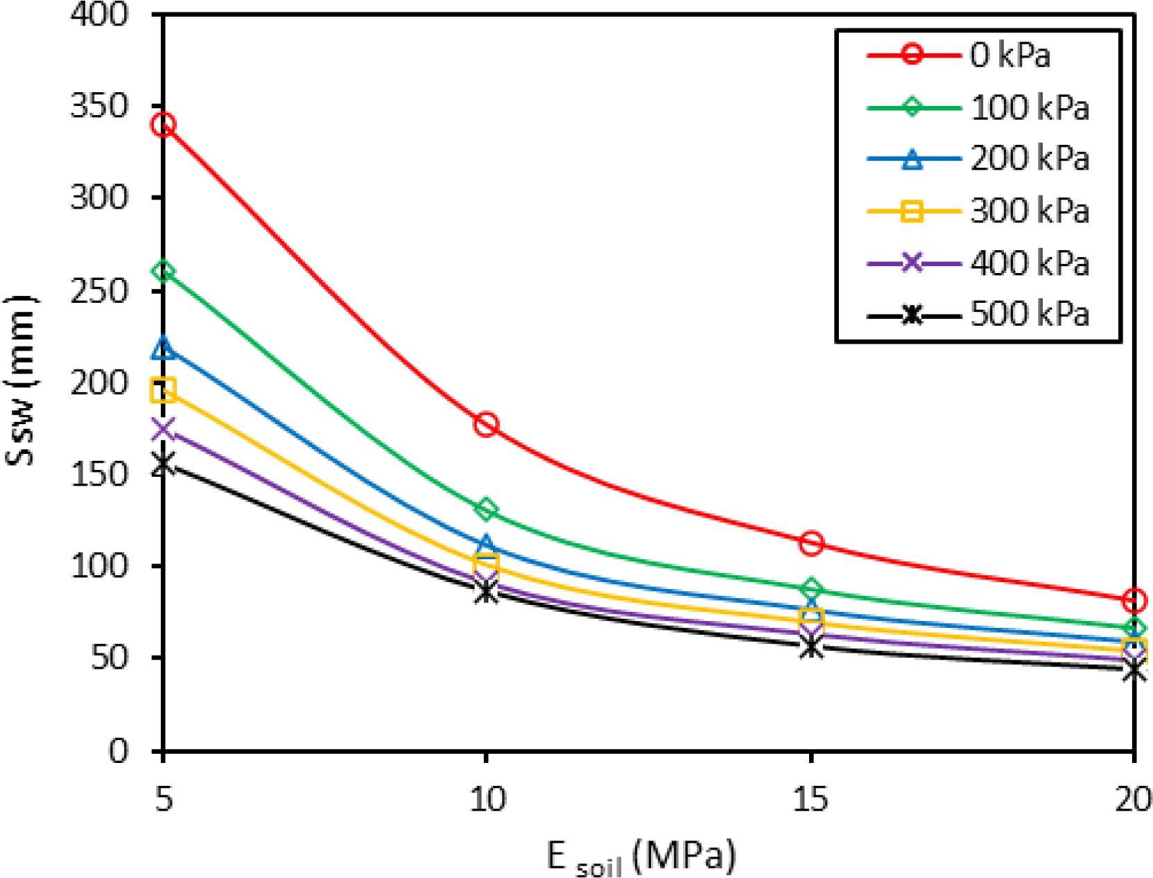
Figure 13
Variation of square footing heave Ssw of width B=1m with soil stiffness Esoil for σ0=0 to 500 kPa.
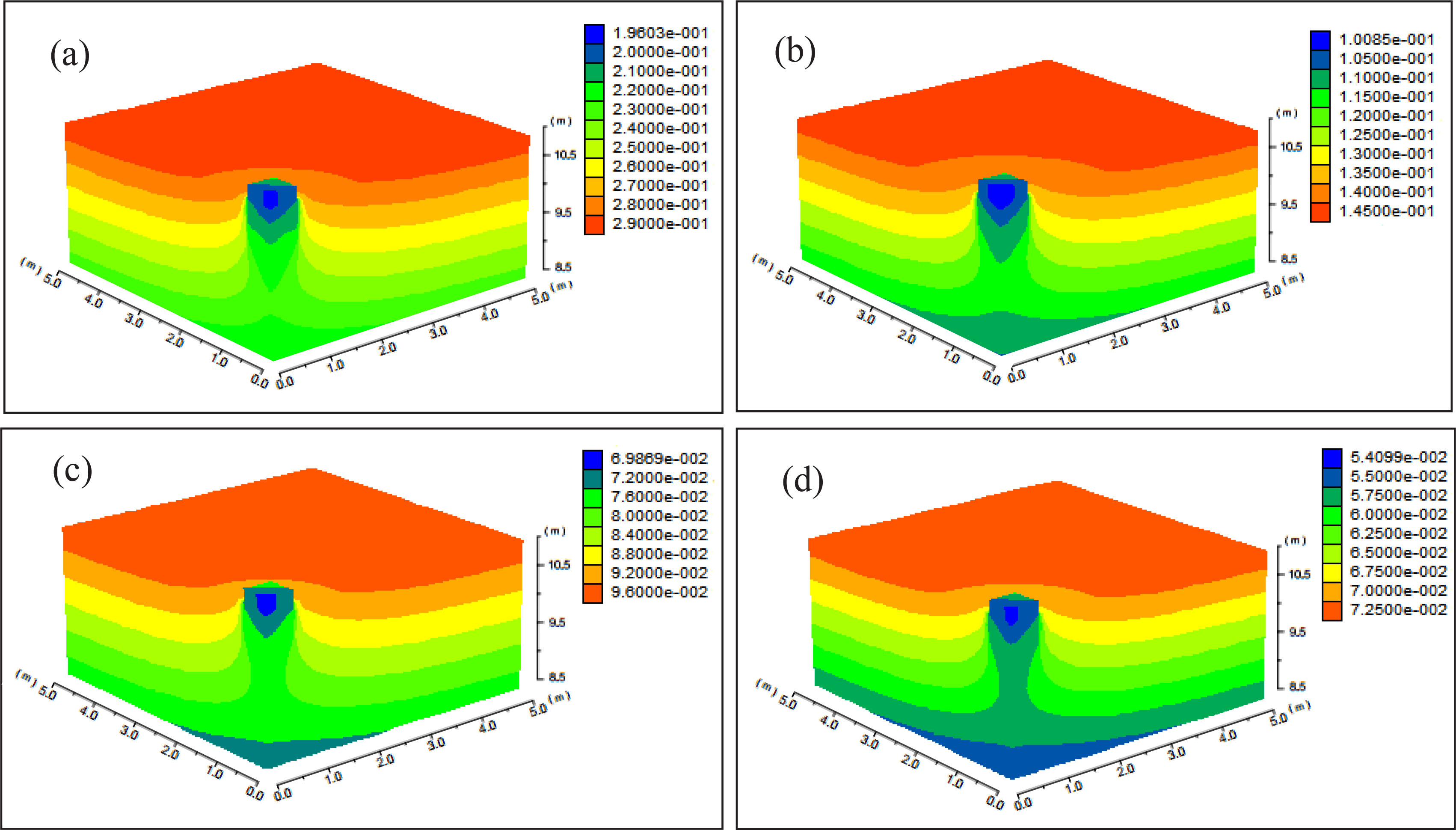
Figure 14
Contours heaving of square footing of width B=1m and σ0=300 kPa with Esoil variation: (a) Esoil=5 MPa, (b) Esoil=10 MPa, (c) Esoil=15 MPa, (d) Esoil=20 MPa.