
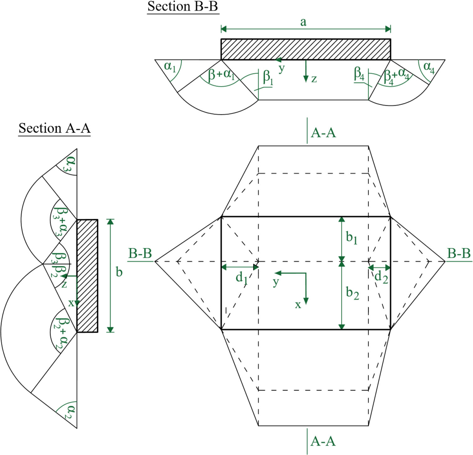
Figure 1
Failure geometry for a rough foundation base in the case of rectangular foundation. More details on failure geometry can be found in Chwała (2019a).
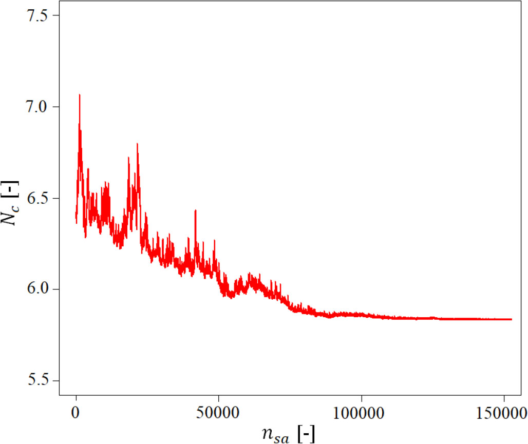
Figure 2
Value of bearing capacity during simulation within optimization procedure
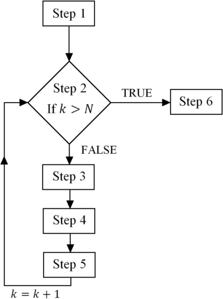
Figure 3
Flow chart of the numerical algorithm. Detailed descriptions of the steps are in the text.
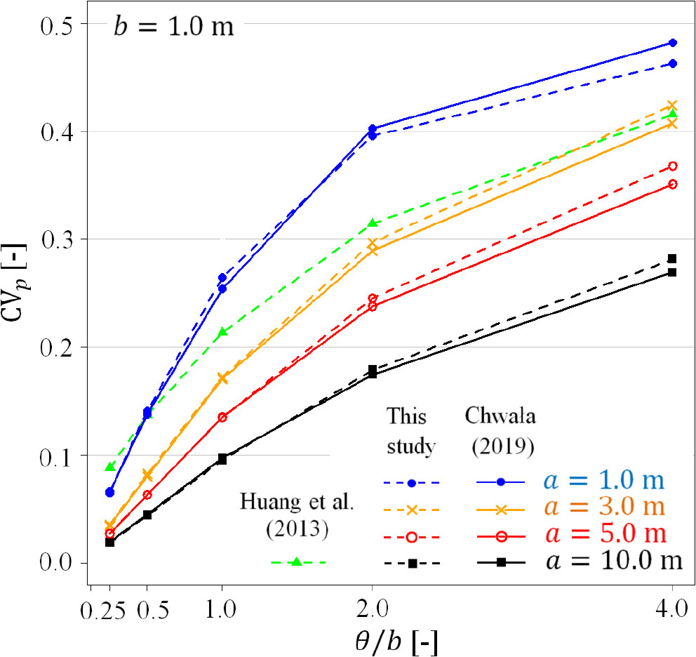
Figure 4
Comparison of bearing capacity variation coefficients obtained by the method proposed in this study (constant covariance matrix) with standard algorithm (individual covariance matrix, Chwała (2019a)). The relative differences between both approaches are below 5%, which is sufficient for the purpose of this study. A detailed description is in the text.
Table 1
Comparison of the results obtained in this study with those obtained by Simoes et al. (2014) by random finite limit analysis.
| Scenario | Method | μNc [-] | σNc [-] | COVNc [-] |
|---|---|---|---|---|
| COVcu=0.5 | RFLA (Simoes et al. 2014) | 4.77 | 1.68 | 0.35 |
| θ=8.0 m | This study | 5.19 | 2.14 | 0.41 |
| COVcu=1.0 | RFLA (Simoes et al. 2014) | 3.72 | 1.23 | 0.33 |
| θ=2.0 m | This study | 4.51 | 1.77 | 0.39 |
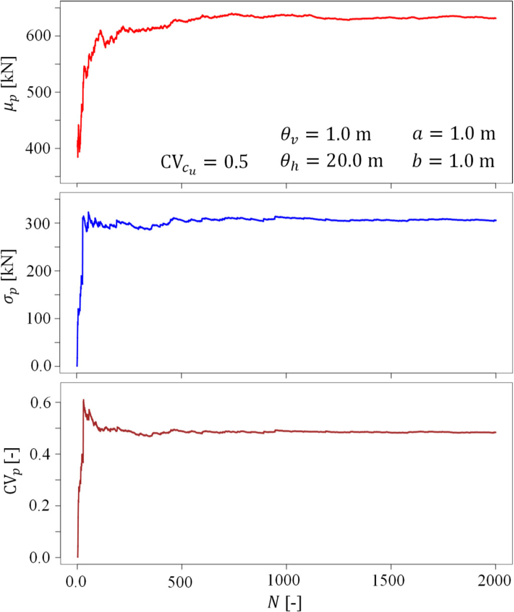
Figure 5
Mean value, standard deviation and variation coefficient of bearing capacity as a function of simulation number N. The square foundation is assumed with geometry parameters and fluctuation scales detailed in the figure.
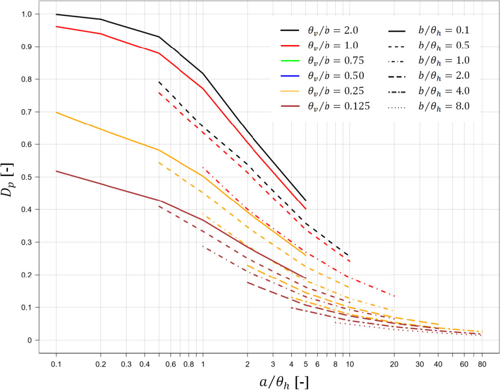
Figure 6
Graph for reading Dp value for ratios θv ⁄ b ∈ [2.0,1.0] and θv ⁄ b∈ [0.25,0.125]. Note that the colour in the legend indicates θv ⁄ b and the line type (coloured on black in the legend) indicates θv ⁄ b.
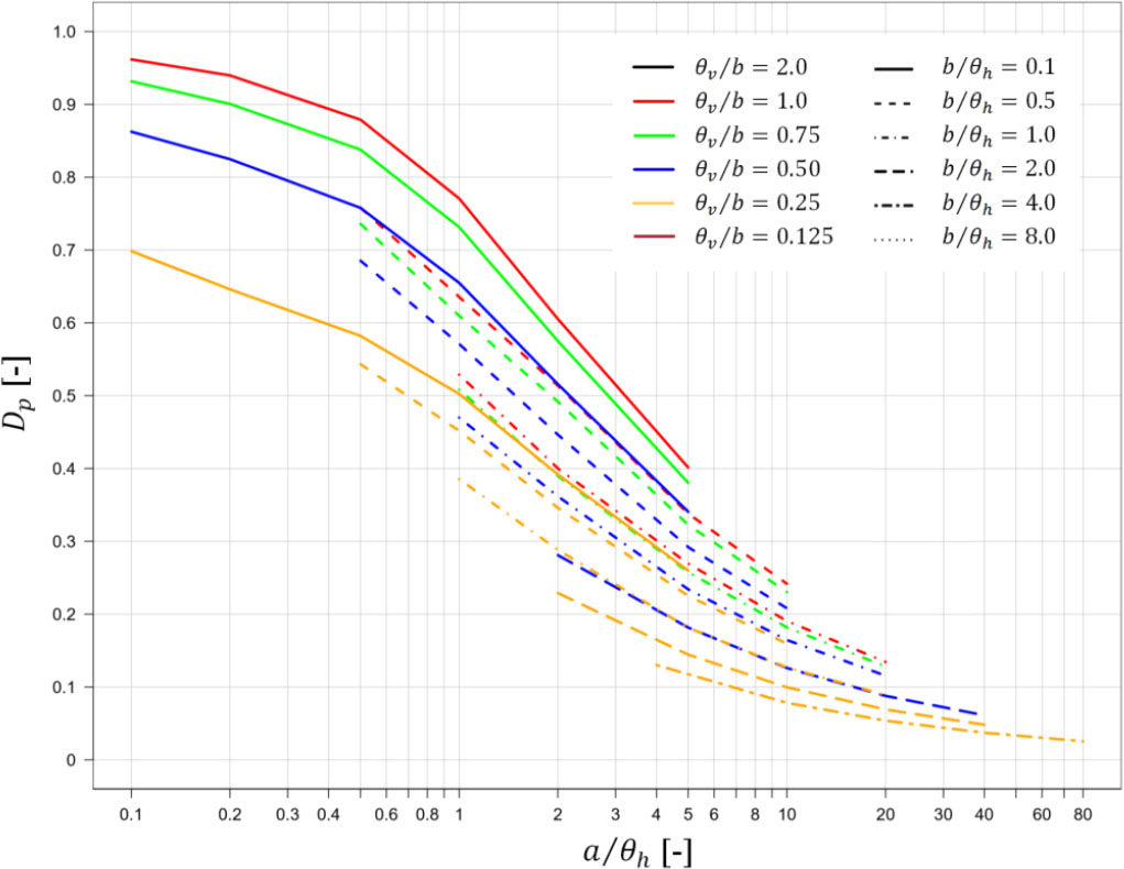
Figure 7
Graph for reading Dp value for ratios θv ⁄ b ∈ [1.0,0.25]. Note that the colour in the legend indicates θv ⁄ b and the line type (coloured on black in the legend) indicates θv ⁄ b.
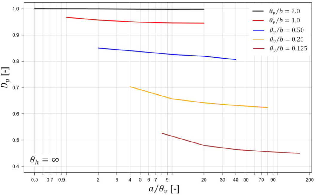
Figure 8
Graph for reading Dp value for an infinite horizontal fluctuation scale.
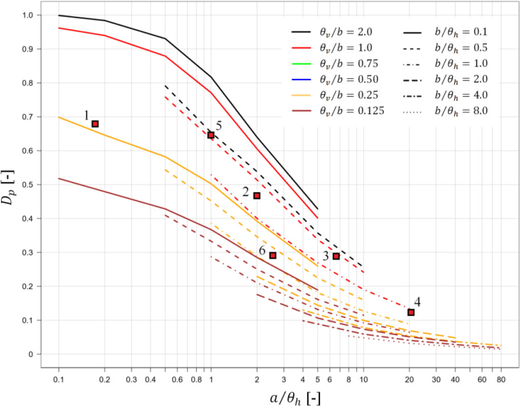
Figure 9
Illustration of example scenarios. Note that the colour in the legend indicates θv ⁄ b and the line type (coloured on black in the legend) indicates θv ⁄ b.
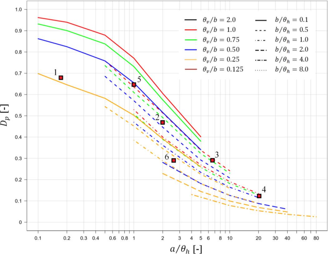
Figure 10
Illustration of example scenarios. Note that the colour in the legend indicates θv ⁄ b and the line type (coloured on black in the legend) indicates θv ⁄ b.
Table 2
Exemplary usage of the graphs proposed in this study. Detailed descriptions are in the text.
| No. | Scenario description | COVp read from graphs [-] | COVp determined by numerical analyses [-] | Difference [%] | ||||
|---|---|---|---|---|---|---|---|---|
| a [m] | b [m] | θv [m] | θh [m] | COVcu [-] | ||||
| 1 | 2.0 | 2.0 | 0.6 | 12.0 | 0.6 | 0.41 | 0.435 | −6.1% |
| 2 | 10.0 | 1.5 | 1.0 | 5.0 | 0.4 | 0.226 | 0.210 | +7.1% |
| 3 | 20.0 | 0.9 | 0.8 | 3.0 | 1.0 | 0.29 | 0.311 | −7.2% |
| 4 | 25.0 | 1.8 | 1.2 | 1.2 | 0.5 | 0.057 | 0.052 | +8.7% |
| 5 | 2.0 | 1.0 | 1.5 | 2.0 | 0.7 | 0.451 | 0.458 | −1.5% |
| 6 | 25.0 | 3.0 | 0.5 | 10.0 | 1.0 | 0.29 | 0.280 | +3.4% |
| 7 | 3.0 | 3.0 | 0.40 | ∞ | 0.24 | 0.13 | 0.130 | 0.0% |
| 8 | 20.0 | 1.0 | 0.47 | ∞ | 0.51 | 0.40 | 0.403 | −0.7% |
Table A.1
Coefficients from Eq. (A.2)–Eq. (A.5) for rough and smooth foundation base. Note that the undrained shear strengths ci are defined individually for each dissipation region (for more details see Chwała, 2019a).
| Coeff. | Expression |
|---|---|
| m1 | c1 cot β2 + 2c21(α2 + β2) + c2 cot α2 |
| m2 | c6 cot α2 + 2c24(α2 + β2) + c5 cot β2 |
| m3 | c8 cot α2 + 2c23(α2 + β2) + c7 cot β2 |
| m4 | c3 cot β3 + 2c22(α3 + β3) + c4 cot α3 |
| m5 | c10 cot α3 + 2c26(α3 + β3) + c9 cot β3 |
| m6 | c12 cot α3 + 2c25(α3 + β3) + c11 cot β3 |
| m7 | c16 cot α1 + 2c28(α1 + β1) + c14 cot β1 |
| m8 | c15 cot α1 + 2c27(α1 + β1) + c13 cot β1 |
| m9 | c20 cot α4 + 2c30(α4 + β4) + c19 cot β4 |
| m10 | c18 cot α4 + 2c29(α4 + β4) + c17 cot β4 |
| n1 | |
| n2 | |
| n3 | |
| n4 | |
| n5 | |
| n6 | |
| n7 | |
| n8 |