
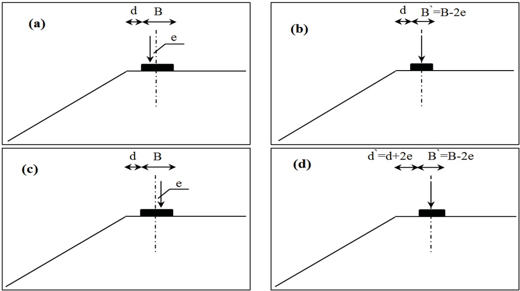
Figure 1
Schematic view of footing model considering the effective width of footing.
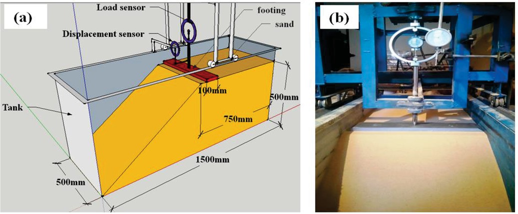
Figure 2
Laboratory model test.
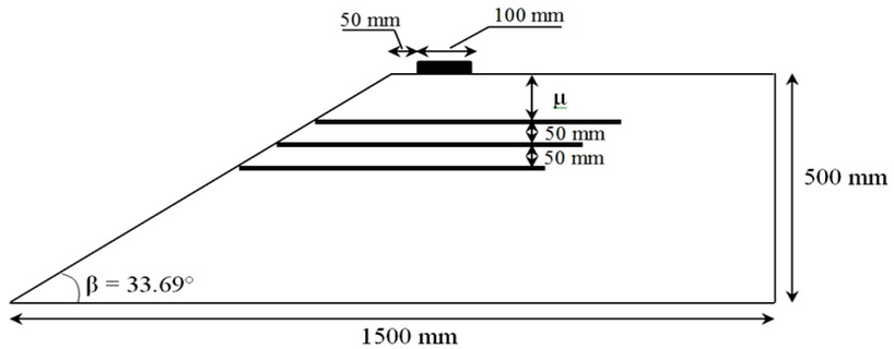
Figure 3
Cross section of model test in the case of reinforced ground by geotextiles.
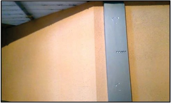
Figure 4
Tested footing with location of applied load.
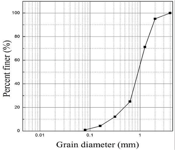
Figure 5
Grain size distribution of tested sand.
Table 1
Material properties of the sand used.
| Parameters | Values |
|---|---|
| Cohesion, c (kPa) | 0.0 |
| Angle of internal friction (°) | 41 |
| Dry unit weight (kN/m3) | 16.1 |
| Maximum dry density (kN/m3) | 19.1 |
| Minimum dry density (kN/m3) | 13.75 |
| D10 | 0.28 |
| D60 | 1.20 |
| D30 | 0.79 |
| Coefficient of uniformity, Cu | 4.28 |
| Coefficient of curvature, Cc | 1.85 |
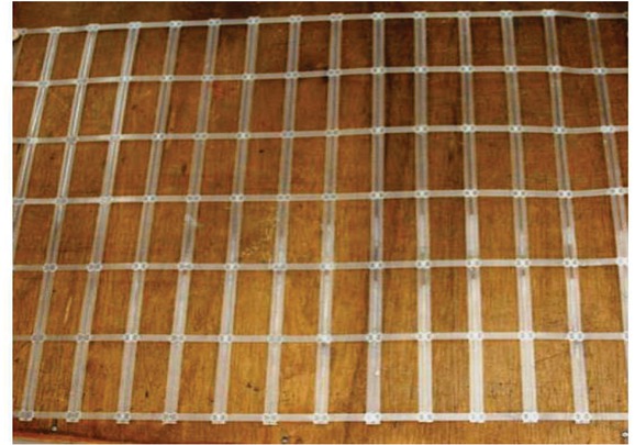
Figure 6
View of geogrid reinforcement.
Table 2
Geogrid properties.
| Description | R6 80/20 |
|---|---|
| Raw material | Transparent polyester |
| Surface ground (g/m2) | 380 |
| Tensile strength (kN/m) | 20 ≤ RT ≤ 80 |
| Elongation (%) | 0 ≤ ΔL ≤ 8 |
| Tensile strength for 1% elongation (kN/m) | 16 |
| Tensile strength for 2% elongation (kN/m) | 28 |
| Tensile strength for 5% elongation (kN/m) | 56 |
| Meshes opening (mm ´ mm) | 73 ´ 30 |
| Elongation before service (%) | 0 |
| Roller dimensions, length and width (m ´ m) | 4.75 ´ 100 |
Table 3
Parameters and conditions of performed tests.
| Test reference | N | μ/B | e/B | d/B |
|---|---|---|---|---|
| C0 | 0 | 0 | 0.5 | |
| T01, F01 | 0.1 | |||
| T02, F02 | 0.2 | |||
| T03, F03 | 0.3 | |||
| C250 | 1 | 0.25 | 0 | |
| T251, F251 | 0.1 | |||
| T252, F252 | 0.2 | |||
| T253, F253 | 0.3 | |||
| C500 | 0.5 | 0 | ||
| T501, F501 | 0.1 | |||
| T502, F502 | 0.2 | |||
| T503, F503 | 0.3 | |||
| C750 | 0.75 | 0 | ||
| T751, F751 | 0.1 | |||
| T752, F752 | 0.2 | |||
| T753, F753 | 0.3 |
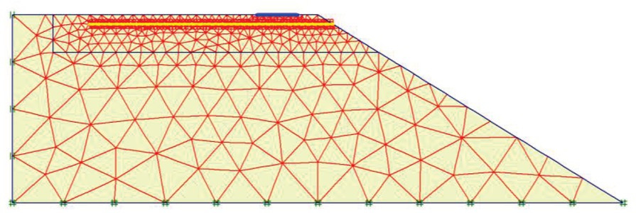
Figure 7
Geometry and mesh size of the numerical model.
Table 4
Parameters used in the numerical study.
| Material | γunsat (kN/m3) | γsat (kN/m3) | E (kn) | ν | EA (kPa) | EI (kN.m2) | φ(°) | ψ(°) | R |
|---|---|---|---|---|---|---|---|---|---|
| Sand | 16.1 | 19.12 | 14,000 | 0.3 | – | – | 41 | 8 | 0.7 |
| Geogrid | – | – | – | 500 | – | – | – | – | |
| Foundation | – | – | – | – | 2.10E+07 | 1.75E+03 | – | – | – |
| – |
Table 5
Ultimate loads of footing under various load eccentricities located towards the slope face.
| N | μ/B | e/B | qu(kN/ml) | iB ;total width | iB ;effective width | ||
|---|---|---|---|---|---|---|---|
| Experimental results | Numerical results using total width method | Numerical results using effective width method | |||||
| 0 | 0 | 2.71 | 2.81 | 2.81 | 1.000 | 1.000 | |
| 0.1 | 1.78 | 1.96 | 2.02 | 0.698 | 0.719 | ||
| 0.2 | 1.38 | 1.5 | 1.54 | 0.534 | 0.548 | ||
| 0.3 | 0.98 | 1.06 | 1.11 | 0.377 | 0.395 | ||
| 1 | 0.25 | 0 | 2.81 | 3.13 | 3.13 | 1.000 | 1.000 |
| 0.1 | 2.53 | 2.66 | 2.75 | 0.850 | 0.879 | ||
| 0.2 | 1.93 | 2.06 | 2.08 | 0.658 | 0.665 | ||
| 0.3 | 1.22 | 1.32 | 1.45 | 0.422 | 0.463 | ||
| 0.4 | 0.64 | 0.66 | 0.204 | 0.211 | |||
| 0.5 | 0 | 3.08 | 3.18 | 3.18 | 1.000 | 1.000 | |
| 0.1 | 2.61 | 2.76 | 2.81 | 0.868 | 0.884 | ||
| 0.2 | 1.78 | 1.88 | 1.91 | 0.591 | 0.601 | ||
| 0.3 | 0.95 | 1.06 | 1.11 | 0.333 | 0.349 | ||
| 0.75 | 0 | 3.11 | 3.2 | 3.2 | 1.000 | 1.000 | |
| 0.1 | 2.24 | 2.42 | 2.55 | 0.756 | 0.797 | ||
| 0.2 | 1.53 | 1.42 | 1.52 | 0.444 | 0.475 | ||
| 0.3 | 0.88 | 0.97 | 1.02 | 0.303 | 0.319 | ||
Table 6
Ultimate loads of footing under various load eccentricities located opposite to the slope face.
| N | μ/B | e/B | qu(kN/ml) | iB ; total width | iB ; effective width | ||
|---|---|---|---|---|---|---|---|
| Experimental | Numerical results with total | Numerical results with | |||||
| results | width method | effective width method | |||||
| 0 | 0 | 2.71 | 2.81 | 2.81 | 1.000 | 1.000 | |
| 0.1 | 2.33 | 2.46 | 2.51 | 0.875 | 0.893 | ||
| 0.2 | 2.08 | 2.02 | 2.1 | 0.719 | 0.747 | ||
| 0.3 | 1.54 | 1.61 | 1.7 | 0.573 | 0.605 | ||
| 1 | 0.25 | 0 | 2.81 | 3.13 | 3.13 | 1.000 | 1.000 |
| 0.1 | 2.55 | 2.7 | 2.83 | 0.863 | 0.904 | ||
| 0.2 | 2.21 | 2.36 | 2.44 | 0.754 | 0.780 | ||
| 0.3 | 1.61 | 1.82 | 1.93 | 0.581 | 0.617 | ||
| 0.5 | 0 | 3.08 | 3.18 | 3.18 | 1.000 | 1.000 | |
| 0.1 | 3 | 3.16 | 3.22 | 0.994 | 1.013 | ||
| 0.2 | 2.75 | 2.87 | 2.96 | 0.903 | 0.931 | ||
| 0.3 | 1.98 | 2.1 | 2.15 | 0.660 | 0.676 | ||
| 0.75 | 0 | 3.11 | 3.2 | 3.2 | 1.000 | 1.000 | |
| 0.1 | 3.1 | 3.23 | 3.27 | 1.009 | 1.022 | ||
| 0.2 | 2.52 | 2.66 | 2.71 | 0.831 | 0.847 | ||
| 0.3 | 1.28 | 1.39 | 1.48 | 0.434 | 0.463 | ||
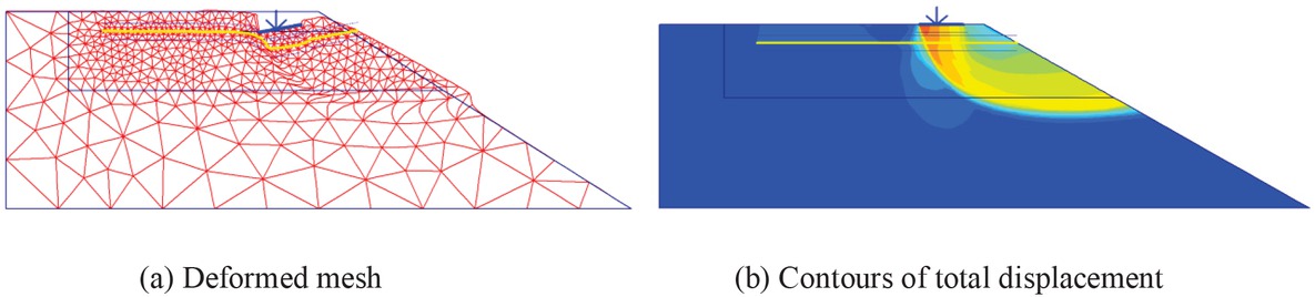
Figure 8
Outputs of PLAXIS code for e/B = 0.1 opposite to the slope facing. (a) Deformed mesh; (b) contours of total displacement.
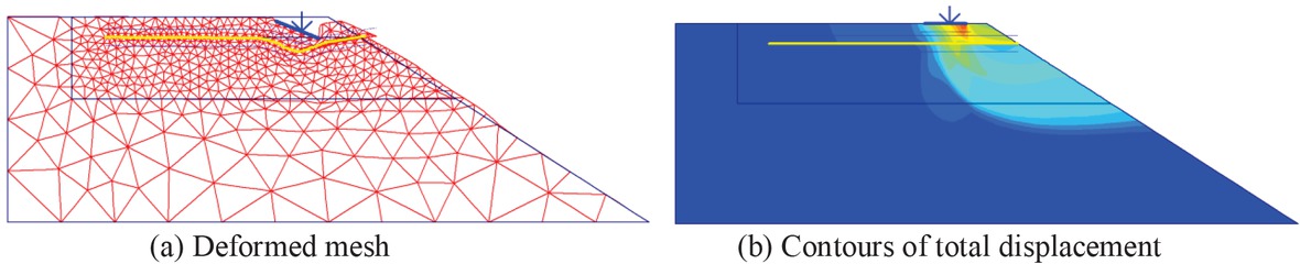
Figure 9
Outputs of PLAXIS code for e/B = 0.1 towards the slope facing. (a) Deformed mesh; (b) contours of total displacement.
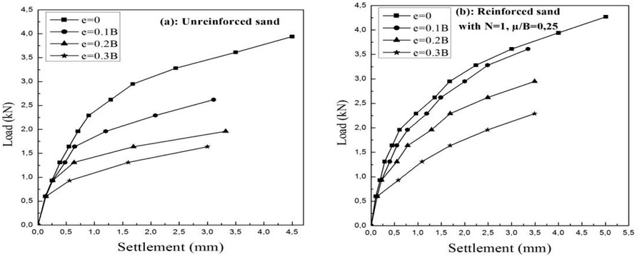
Figure 10
Relationship between the failure load and the displacements of a strip footing under various eccentricities located towards the reinforced slope face.
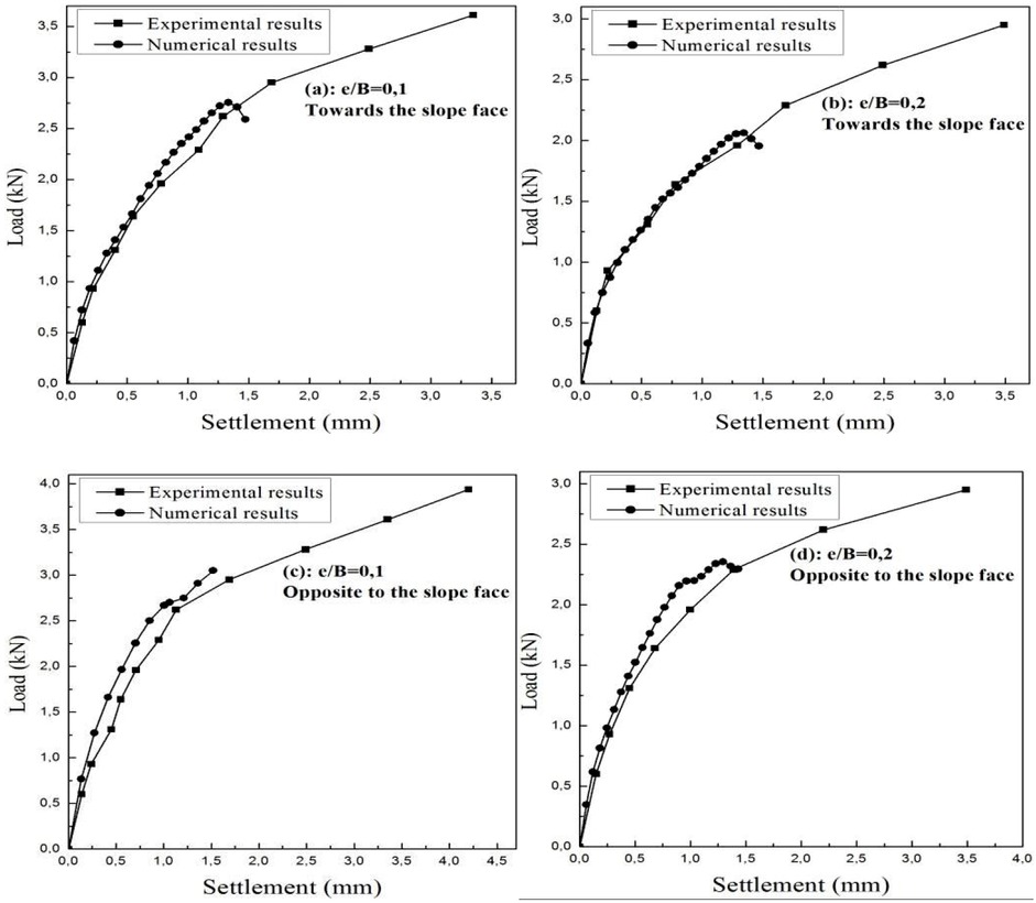
Figure 11
Comparison between the experimental and numerical results for reinforced sand (N = 1, m/B = 0.25).
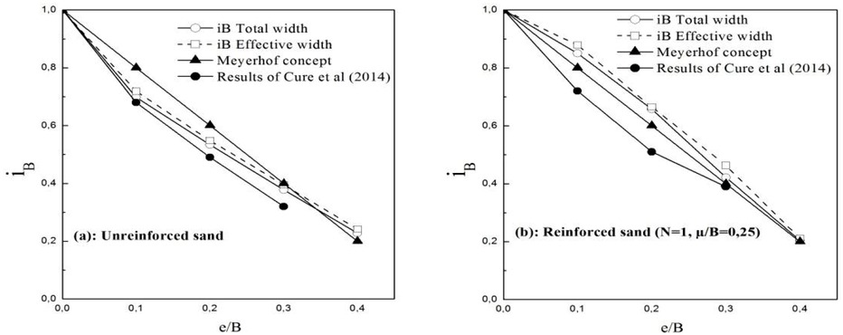
Figure 12
Variation of iB versus e/B of a strip footing under eccentric load located towards the reinforced slope face.
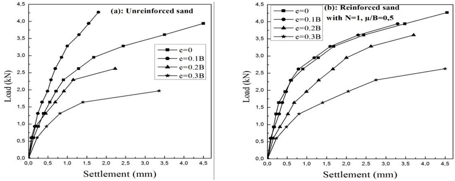
Figure 13
Relationship between the failure load and the displacements of a strip footing under various eccentricities located opposite to the reinforced slope face.
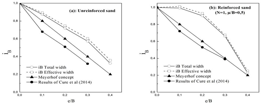
Figure 14
Variation of iB versus e/B of a strip footing under load eccentricity located opposite to the reinforced slope face.
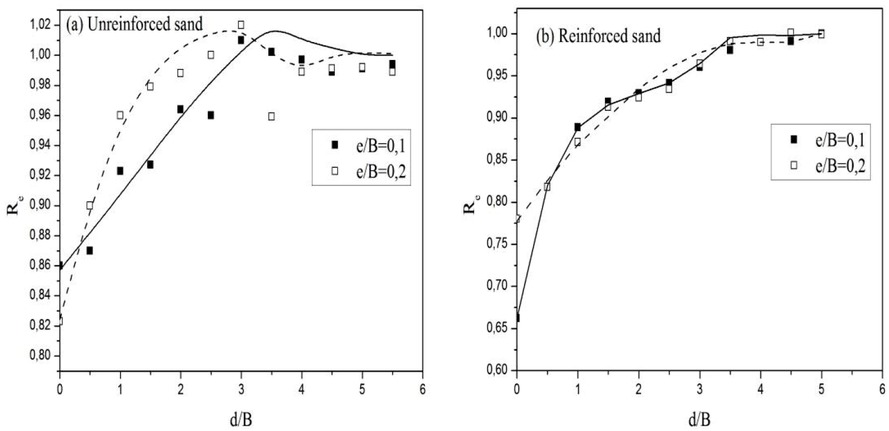
Figure 15
Variation of Re versus d/B.