
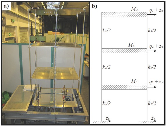
Figure 1
The slab-and-column model: (a) physical; (b) theoretical.
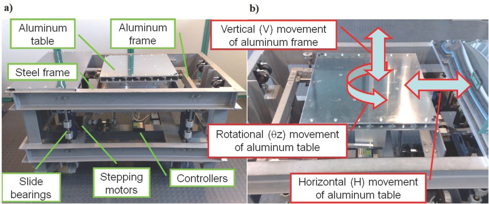
Figure 2
The shake table: (a) main elements and (b) possible directions of kinematic excitation.
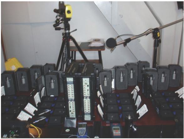
Figure 3
Measurement instruments—PULSE system by Brüel & Kjær.
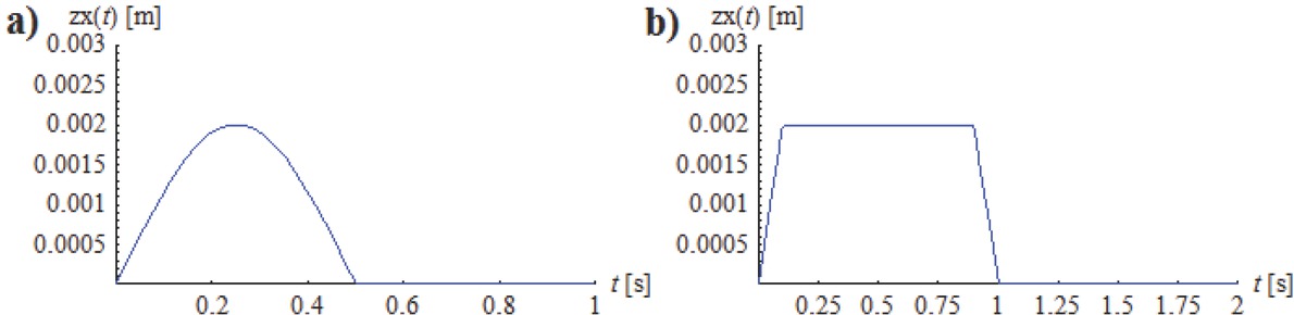
Figure 4
Kinematic excitations: (a) “sine”; (b) “trapezium”.
Table 1
Data on kinematic excitations.
| Measurement No. | Name of excitation | Amplitude of excitation (mm) | Time duration of excitation (s) |
|---|---|---|---|
| 1 | “sine” | 2 | 0.5 |
| 2 | “sine” | 4 | 0.5 |
| 3 | “trapezium” | 2 | 1 |
| 4 | “trapezium” | 4 | 1 |
| 5 | “trapezium” | 2 | 2 |
| 6 | “trapezium” | 4 | 2 |
Table 2
Key results of experimental research.
| Measurement | |||||||
|---|---|---|---|---|---|---|---|
| No. 1 | No. 2 | No. 3 | No. 4 | No. 5 | No. 6 | ||
| Values of limit expressions—formulas (11, 12) | Y1c | 249.353 | 496.455 | 422.826 | 843.34 | 401.447 | 788.547 |
| (mm) | |||||||
| Y2c | 349.069 | 695.045 | 591.967 | 1,180.66 | 562.036 | 1,103.95 | |
| (mm) | |||||||
| Y3c | 398.909 | 794.343 | 676.542 | 1,349.31 | 642.335 | 1,261.64 | |
| (mm) | |||||||
| Zc | 6,283.19 | 12,566.4 | 10,000.0 | 20,000.0 | 10,000.0 | 20,000.0 | |
| (mm/s2) | |||||||
| Coefficients of the stiffness matrix have been determined based on formula (13) | k1 | 1,037.6 | 1,042.31 | 973.876 | 976.546 | 1,025.74 | 1,044.4 |
| (N/m) | |||||||
| k2 | 1,918.93 | 1,927.07 | 1,800.51 | 1,805.64 | 1,896.4 | 1,931.1 | |
| (N/m) | |||||||
| k3 | 2,561.7 | 2,571.53 | 2,402.58 | 2,409.76 | 2,530.53 | 2,577.21 | |
| (N/m) | |||||||
| Natural frequencies of the model have been determined based on formulas (14, 15) | f1 | 0.665 | 0.667 | 0.644 | 0.645 | 0.661 | 0.667 |
| (Hz) | |||||||
| f2 | 2.343 | 2.349 | 2.270 | 2.274 | 2.330 | 2.351 | |
| (Hz) | |||||||
| f3 | 3.929 | 3.937 | 3.806 | 3.811 | 3.906 | 3.942 | |
| (Hz) |
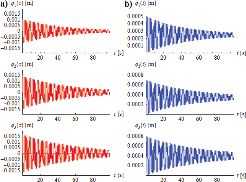
Figure 5
The results obtained from the first measurement: (a) displacement plots in the time domain t and (b) displacements determined in accordance with formula (7).
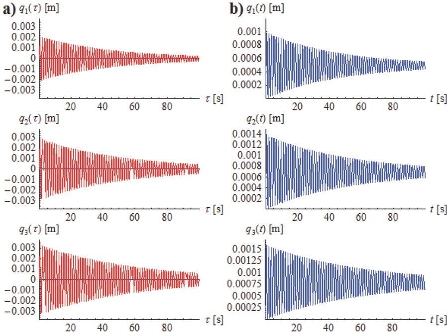
Figure 6
Results obtained from the second measurement: (a) displacement plots in the time domain t; and b) displacements determined in accordance with formula (7).
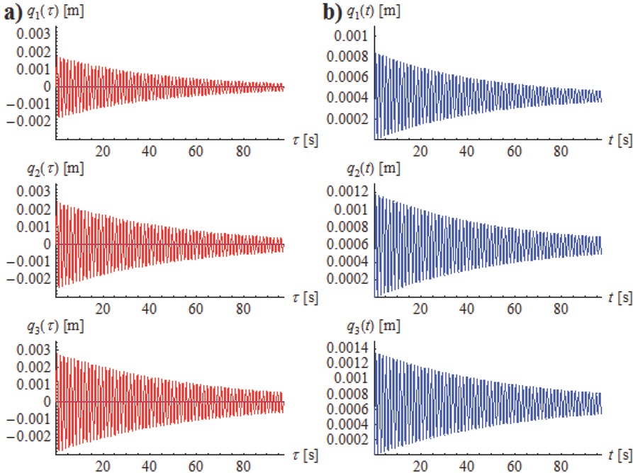
Figure 7
The results obtained from the third measurement: (a) displacement plots in the time domain t and (b) displacements determined in accordance with formula (7).
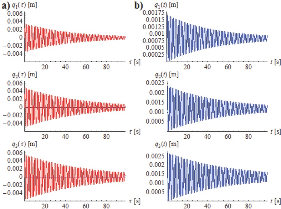
Figure 8
The results obtained from the fourth measurement: (a) displacement plots in the time domain t and (b) displacements determined in accordance with formula (7).
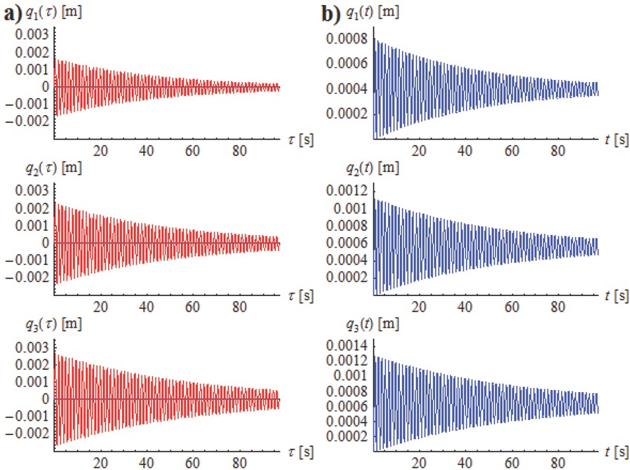
Figure 9
The results obtained from the fifth measurement: (a) displacement plots in the time domain t and (b) displacements determined in accordance with formula (7).
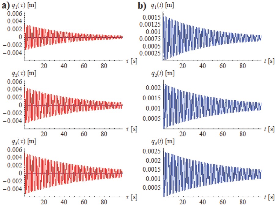
Figure 10
The results obtained from the sixth measurement: (a) displacement plots in the time domain t and (b) displacements determined in accordance with formula (7).