
Table 1:
Outcome Variables and Covariates
| Variables | Description |
|---|---|
| Outcome variables | |
| Food expenditure | (Amount of food expenses) |
| Transport expenditure | (Amount of transport expenditure) |
| Household income | (Household income) |
| Health expenditure | (Amount of health expenditure) |
| Clothing expenditure | (Amount of closing expenditure) |
| Education expenditure | (Amount of education expenditure) |
| Rent Expenditure | (Amount of rent expenditure) |
| Independent variable | |
| Access to Credit | =1 if a household has access to credit and =0 if no access to credit |
| Covariates | |
| Hhage (years) | Age of the respondent |
| HHsize | Household size |
| Female | Dummy (1= female and 0 =male) |
| Educated | Dummy (1=primary school and above and 0 =not educated |
| Single | Dummy (1= single and 0 =otherwise) |
| Rural | Dummy for the area (1=Rural and 0 =Urban) |
Table 2:
Summary Statistics
| Variables | Treatment group | Control group | Difference |
|---|---|---|---|
| Treatment variable | |||
| Access to credit | 1 | 0 | |
| Outcomes variable | |||
| Transport Expenditure | 184.72 | 113.98 | 70.74 |
| Food Expenditure | 644.12 | 470.19 | 173.93 |
| Household income | 2324.87 | 1420.33 | 904.54 |
| Health Expenditure | 100.04 | 71.41 | 28.63 |
| Closing Expenditure | 54.47 | 15.90 | 38.57 |
| Education Expenditure | 86.71 | 32.46 | 54.25 |
| Rent Expenditure | 131.73 | 64.54 | 67.19 |
| Covariates | |||
| Rural | .59 | .63 | -0.04 |
| Hhage | 49.68 | 51.21 | -1,53 |
| Hhsize | 4.07 | 3.86 | 0,21 |
| Female | .41 | .40 | 0.01 |
| Educatwed | .86 | .87 | -0.01 |
| Single | .15 | .22 | -0.07 |
| Observations | 1,805 | 1,194 | 2,999 |
Table 3:
Impact of access to credit on expenditures
| Outcomes Variable | Nearest neighbor Matching | Caliper Matching | Kernel Matching |
|---|---|---|---|
| Transport Expenditure | 63.75*** | 66.56*** | 66.59*** |
| Food Expenditure | 150.27*** | 157.02*** | 157.04*** |
| Household income | 816.52*** | 850.97*** | 851.26*** |
| Health Expenditure | 28.87*** | 28.56*** | 28.56*** |
| Closing Expenditure | 36.68*** | 37.68*** | 37.68*** |
| Education Expenditure | 50.88*** | 52.06*** | 52.06*** |
| Rent Expenditure | 57.35*** | 63.01*** | 63.03*** |
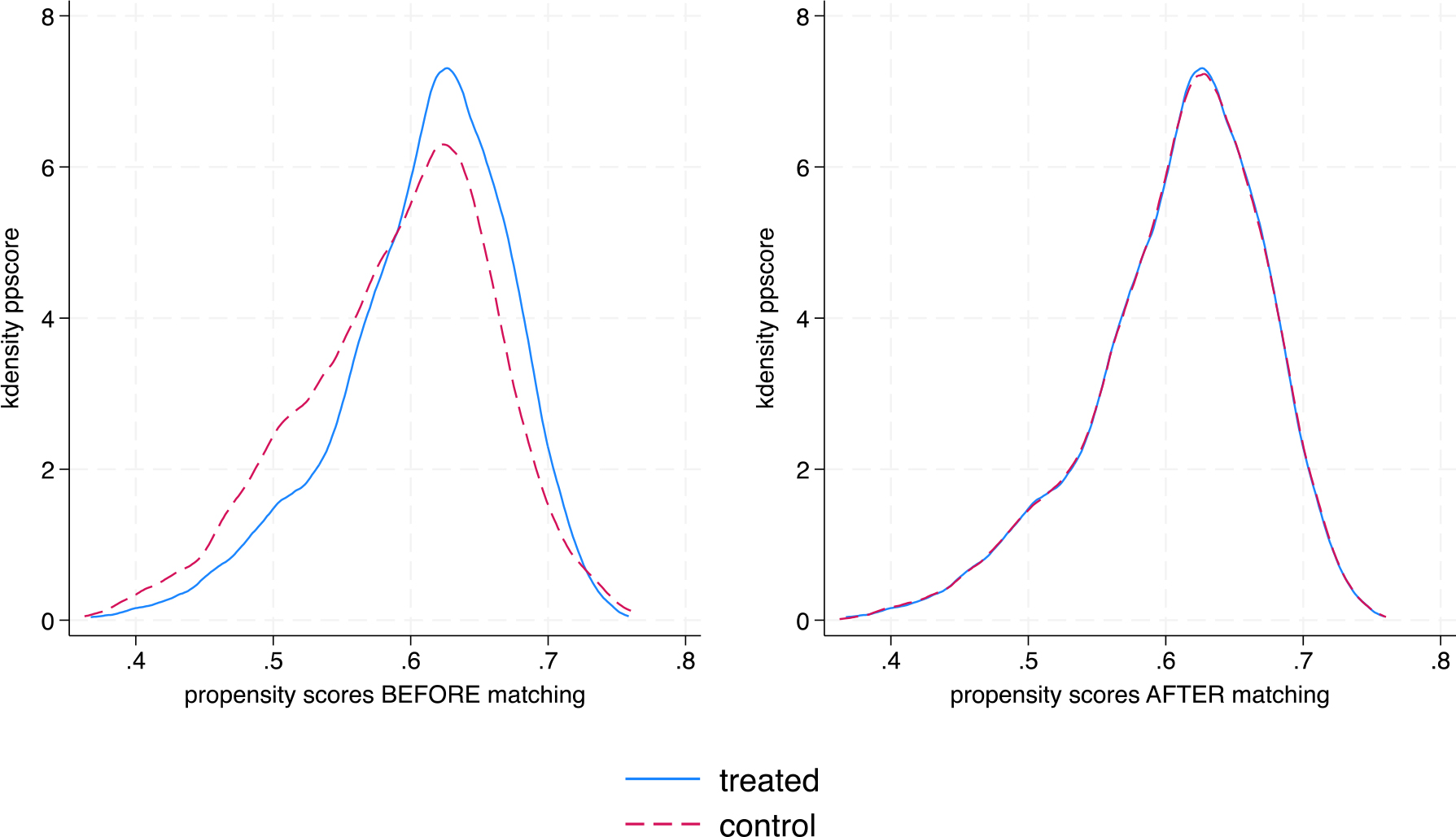
Figure 1:
Distribution of Covariates before and after matching
Both estimation methods (IPWRA and MDM) are consistent with the PSM method. The two techniques indicate that access to credit significantly increases household expenditure and income.
Table 4:
Inverse Probability weighting regression adjustment estimation
| Outcomes variable | IPWRA estimation | MDM estimation |
|---|---|---|
| Transport Expenditure | 64.39*** | 56.28*** |
| Food Expenditure | 157.33*** | 157.98*** |
| Household income | 844.77*** | 785.08*** |
| Health Expenditure | 27.21*** | 25.37*** |
| Closing Expenditure | 38.09*** | 38.40*** |
| Education Expenditure | 51.78*** | 36.64*** |
| Rent Expenditure | 60.62*** | 43.91*** |
Table 5:
Covariates Balance Check
| Mean | |||||
|---|---|---|---|---|---|
| Before matching | Treated | Control | Bias reduction (%) | P-value | |
| Female | .41 | .40 | 0.000 | ||
| Educated | .86 | .87 | 0.000 | ||
| Single | .15 | .22 | 0.000 | ||
| HHsize | 4.07 | 3.86 | 0.011 | ||
| Rural | .59 | .63 | 0.078 | ||
| HHage | 49.68 | 51.21 | 0.017 | ||
| After matching | |||||
| Female | .41 | .41 | 44.3 | 0.561 | |
| Educated | .86 | .86 | 91.2 | 0.938 | |
| Single | .15 | .14 | 84.1 | 0.340 | |
| HHsize | 4.07 | 3.86 | 96.9 | 0.886 | |
| Rural | .59 | .60 | 70.6 | 0.951 | |
| HHage | 49.68 | 50.13 | 95.0 | 0.426 | |