
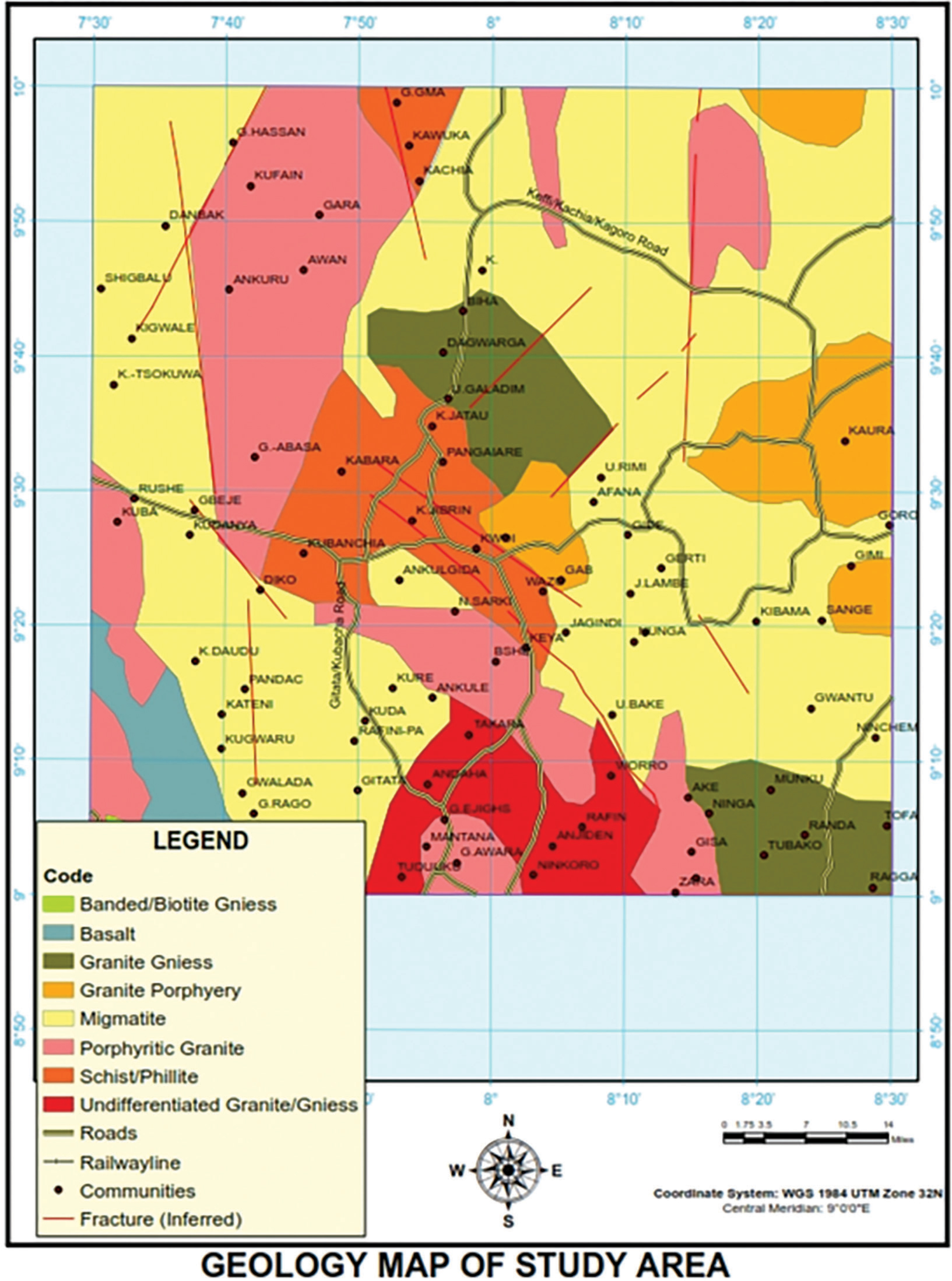
Figure 1:
Geologic map of the study area.
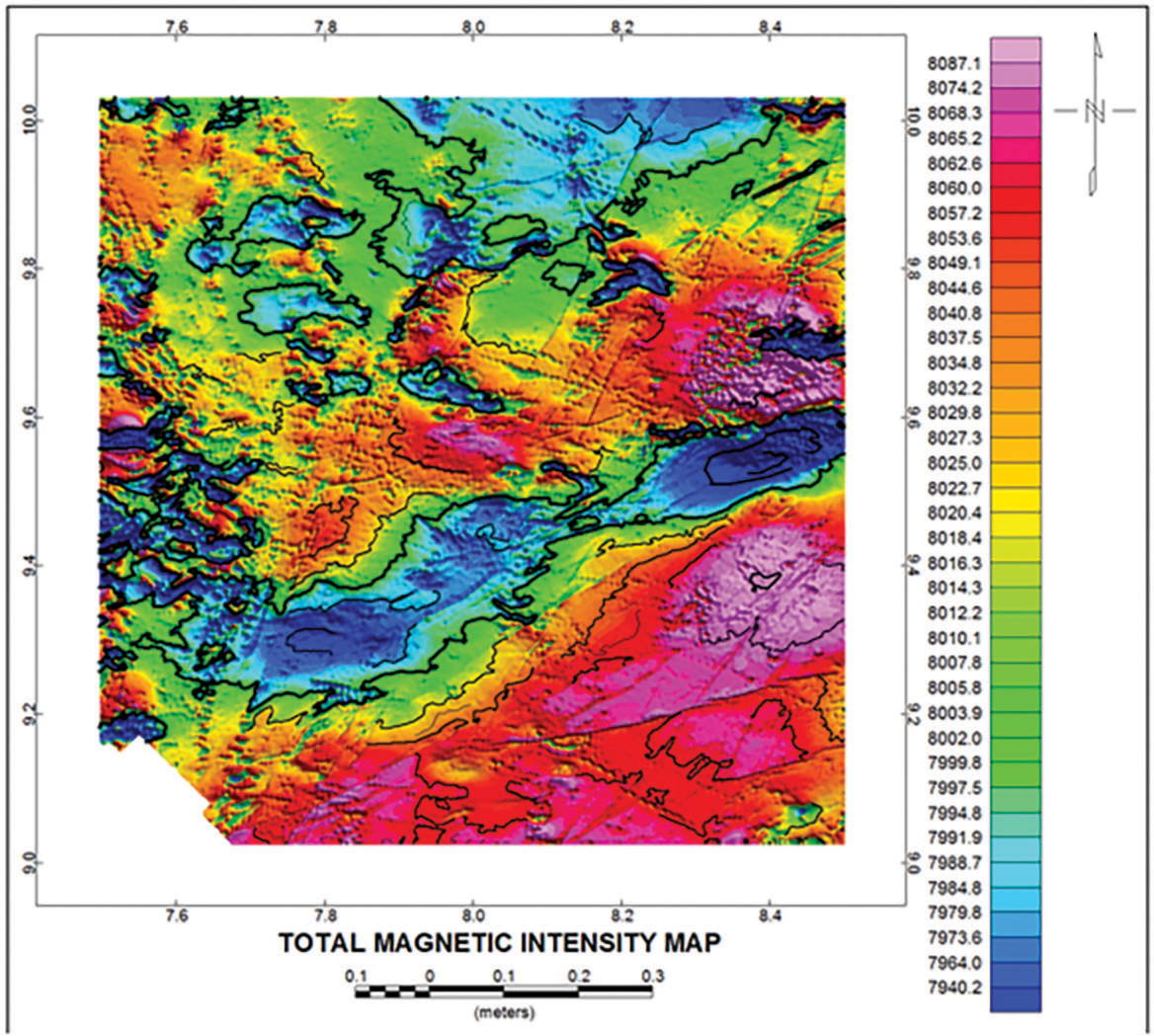
Figure 2:
Aeromagnetic field over the study area as a color-shaded, contoured map.
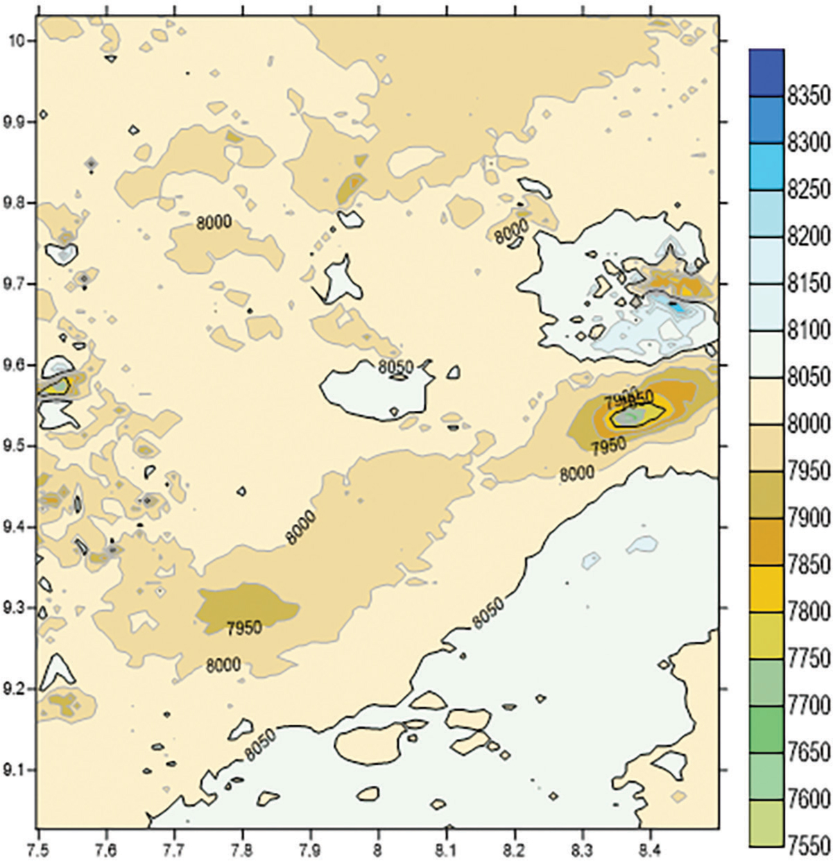
Figure 3:
Color-coded pixel contour map of the total magnetic field of the study area in gammas.
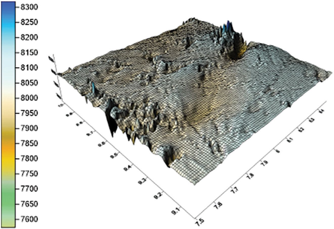
Figure 4:
3-D surface map of the total magnetic field of the study area in gammas.
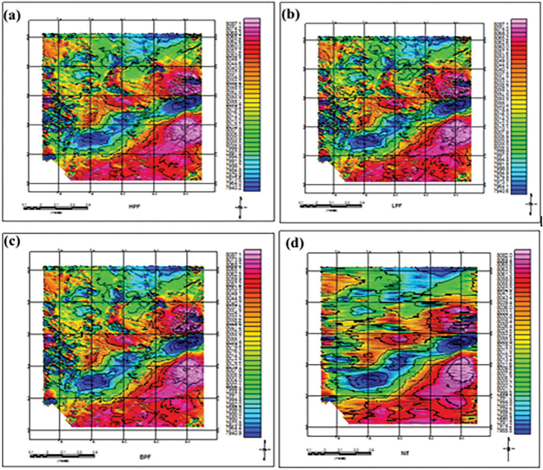
Figure 5:
(a) High-pass filter, (b)low-pass filter, (c) band-pass filter, (d) non-linear filter map of the total magnetic field intensity of the study area.
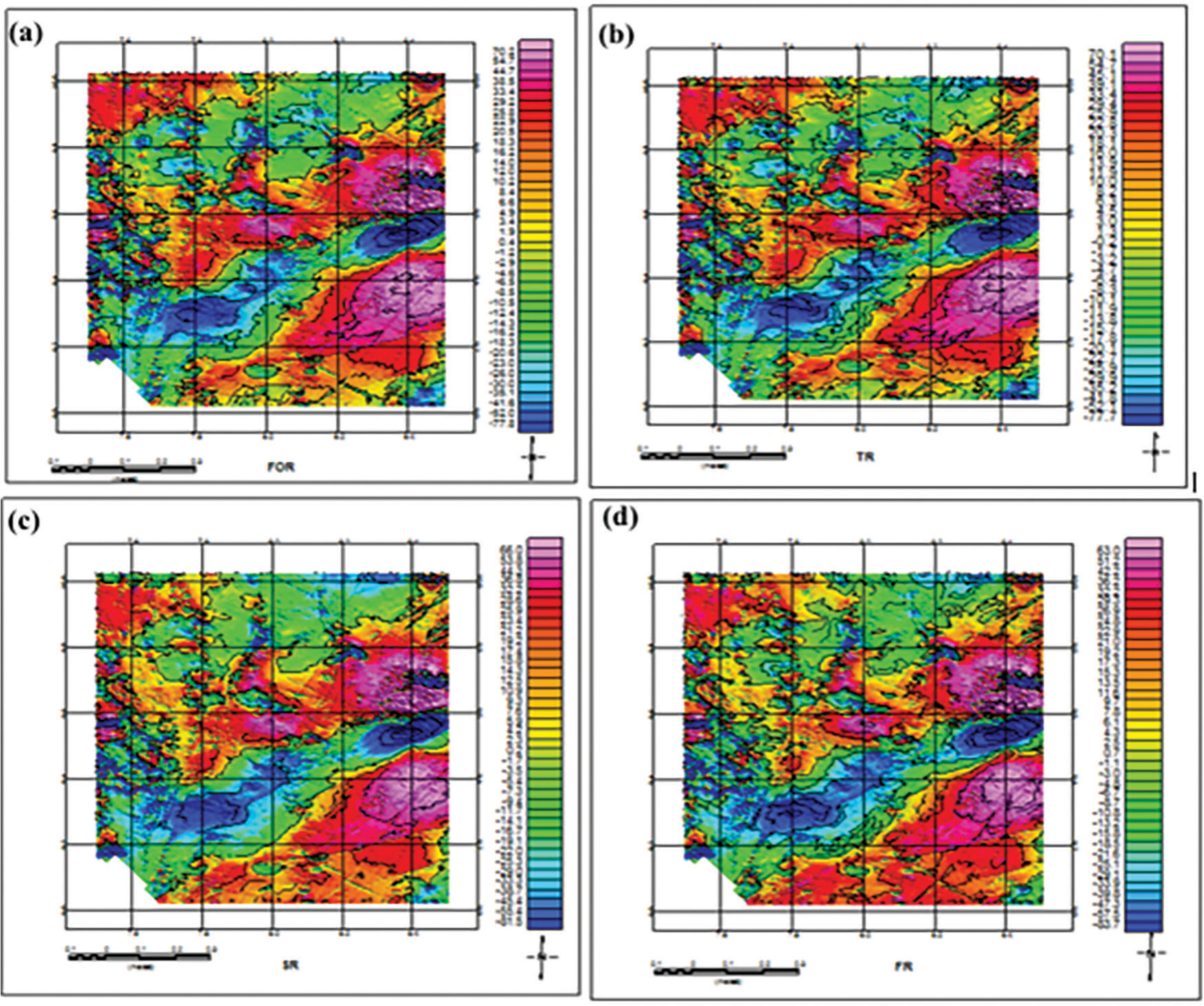
Figure 6:
(a) First-degree residual, (b) second-degree residual, (c) third-degree residual, (d) fourth-degree residual field over the study area as a color-shaded contour map.
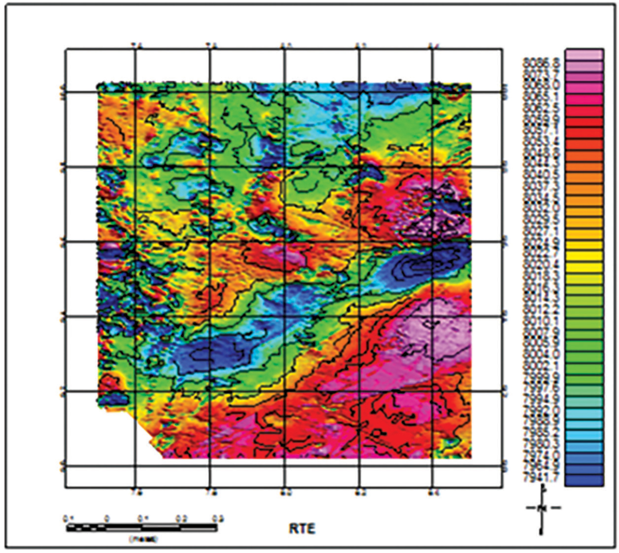
Figure 7:
Reduction to equator of the aeromagnetic field over the study area as a color-shaded, contoured map.
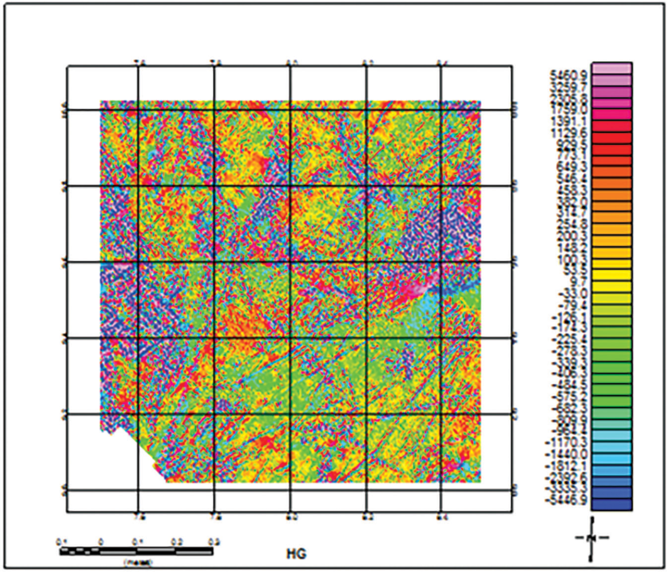
Figure 8:
Horizontal gradient of the aeromagnetic field over the study area as a color-shaded, contoured map.
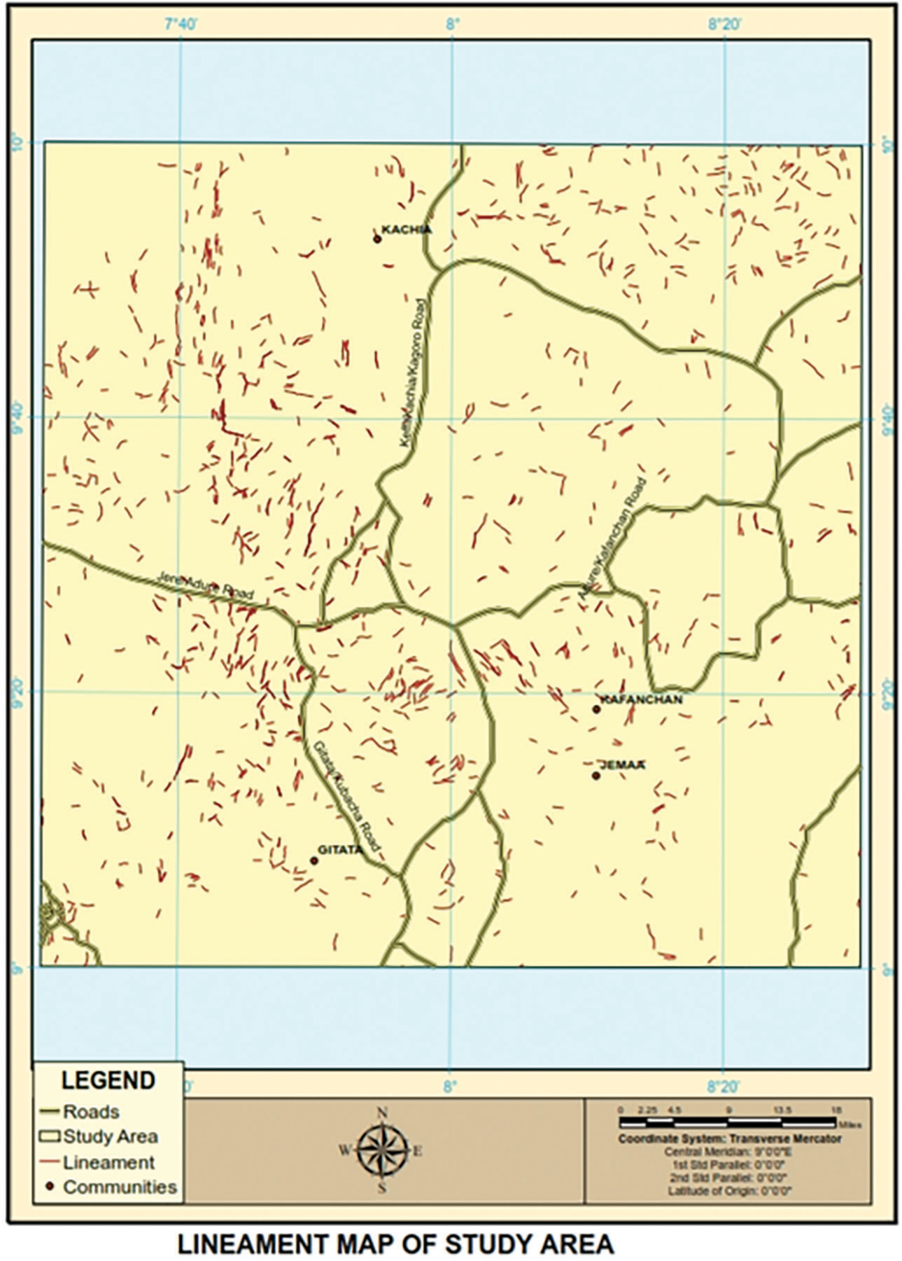
Figure 9:
Lineament map of study area.
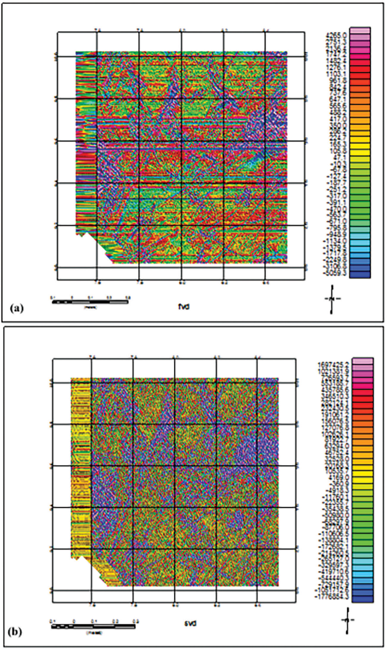
Figure 10:
(a) D1 values (shallow magnetic basement depths) and (b) D2 (basement depths across the study area).
Table 1:
Computed spectral depths.
| Portions | Depth 1 (m) | Depth 2 (m) |
|---|---|---|
| 1 | 136.34 | 1659.50 |
| 2 | 200.53 | 1618.28 |
| 3 | 135.85 | 1585.18 |
| 4 | 136.15 | 2021.74 |
| 5 | 136.37 | 1615.90 |
| 6 | 136.36 | 1864.81 |
| 7 | 136.41 | 1933.89 |
| 8 | 136.39 | 1770.43 |
| 9 | 136.36 | 1655.05 |
| 10 | 136.34 | 1657.43 |
| 11 | 136.30 | 1810.54 |
| 12 | 135.98 | 1784.44 |
| 13 | 136.42 | 1850.81 |
| 14 | 138.17 | 1999.46 |
| 15 | 135.50 | 1756.11 |
| 16 | 135.61 | 1871.02 |
Table 2:
Computed spectral depths in km according to sheets.
| Sheets | Spectra L Block | Longitude | Latitude | Depth (km) | |||
|---|---|---|---|---|---|---|---|
| X1 | X2 | Y1 | Y2 | D1 | D2 | ||
| Kachia | 13 | 7.50 | 7.75 | 9.75 | 10.00 | 0.136 | 1.851 |
| 14 | 7.75 | 8.00 | 9.75 | 10.00 | 0.138 | 1.999 | |
| 9 | 7.50 | 7.75 | 9.50 | 9.75 | 0.136 | 1.655 | |
| 10 | 7.75 | 8.00 | 9.50 | 9.75 | 0.136 | 1.657 | |
| 15 | 8.00 | 8.25 | 9.75 | 10.00 | 0.136 | 1.756 | |
| Kafanchan | 16 | 8.25 | 8.50 | 9.75 | 10.00 | 0.135 | 1.871 |
| 11 | 8.00 | 8.25 | 9.50 | 9.75 | 0.136 | 1.810 | |
| 12 | 8.25 | 8.50 | 9.50 | 9.75 | 0.135 | 1.784 | |
| 5 | 7.50 | 7.75 | 9.25 | 9.50 | 0.136 | 1.616 | |
| Gitata | 6 | 7.75 | 8.00 | 9.25 | 9.50 | 0.136 | 1.864 |
| 1 | 7.50 | 7.75 | 9.00 | 9.25 | 0.136 | 1.660 | |
| 2 | 7.75 | 8.00 | 9.00 | 9.25 | 0.201 | 1.618 | |
| 7 | 8.00 | 8.25 | 9.25 | 9.50 | 0.136 | 1.934 | |
| Jema’a | 8 | 8.25 | 8.50 | 9.25 | 9.50 | 0.136 | 1.770 |
| 3 | 8.00 | 8.25 | 9.00 | 9.25 | 0.136 | 1.585 | |
| 4 | 8.25 | 8.50 | 9.00 | 9.25 | 0.136 | 2.021 | |
Table 3:
Computed spectral depth, Curie temperature and heat flow.
| Longitude | Latitude | CPD (km) | Geothermal Gradient (°Ckm-1) | Heat Flow (mWm-2) | |||||
|---|---|---|---|---|---|---|---|---|---|
| SPECTRAL LINES | X1 | X2 | Y1 | Y2 | Zt | ZO | Zb | dT/dZ | q |
| 1 | 7.50 | 7.75 | 9.00 | 9.25 | 1.660 | 14.354 | 27.048 | 21.44336 | 53.6084 |
| 2 | 7.75 | 8.00 | 9.00 | 9.25 | 1.618 | 15.426 | 29.234 | 14 | 49.5997 |
| 3 | 8.00 | 8.25 | 9.00 | 9.25 | 1.585 | 14.286 | 26.987 | 21.49183 | 53.7296 |
| 4 | 8.25 | 8.50 | 9.00 | 9.25 | 2.022 | 12.950 | 23.878 | 24.2901 | 60.7253 |
| 5 | 7.50 | 7.75 | 9.25 | 9.50 | 1.616 | 13.980 | 26.344 | 22.01639 | 55.0409 |
| 6 | 7.75 | 8.00 | 9.25 | 9.50 | 1.865 | 12.620 | 23.375 | 24.81283 | 62.0321 |
| 7 | 8.00 | 8.25 | 9.25 | 9.50 | 1.934 | 12.120 | 22.306 | 26.00197 | 65.0049 |
| 8 | 8.25 | 8.50 | 9.25 | 9.50 | 1.770 | 12.340 | 22.91 | 25.31646 | 63.2912 |
| 9 | 7.50 | 7.75 | 9.50 | 9.75 | 1.655 | 12.734 | 23.813 | 24.35644 | 60.8911 |
| 10 | 7.75 | 8.00 | 9.50 | 9.75 | 1.657 | 14.320 | 26.983 | 21.49501 | 53.7375 |
| 11 | 8.00 | 8.25 | 9.50 | 9.75 | 1.811 | 14.240 | 26.669 | 21.74809 | 54.3702 |
| 12 | 8.25 | 8.50 | 9.50 | 9.75 | 1.784 | 13.980 | 26.176 | 22.15770 | 55.3943 |
| 13 | 7.50 | 7.75 | 9.75 | 10.00 | 1.851 | 13.410 | 24.969 | 23.22880 | 58.072 |
| 14 | 7.75 | 8.00 | 9.75 | 10.00 | 1.9996 | 13.510 | 25.0204 | 23.18108 | 57.9527 |
| 15 | 8.00 | 8.25 | 9.75 | 10.00 | 1.756 | 13.720 | 25.684 | 22.58215 | 56.4553 |
| 16 | 8.25 | 8.50 | 9.75 | 10.00 | 1.871 | 13.340 | 24.809 | 23.37861 | 58.4465 |
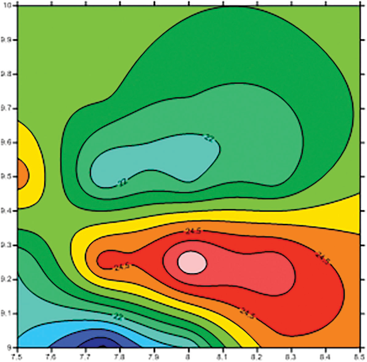
Figure 11:
Plot of the geothermal gradient of the study area.
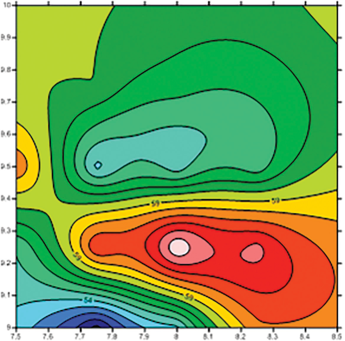
Figure 12:
Plot of the heat flow.
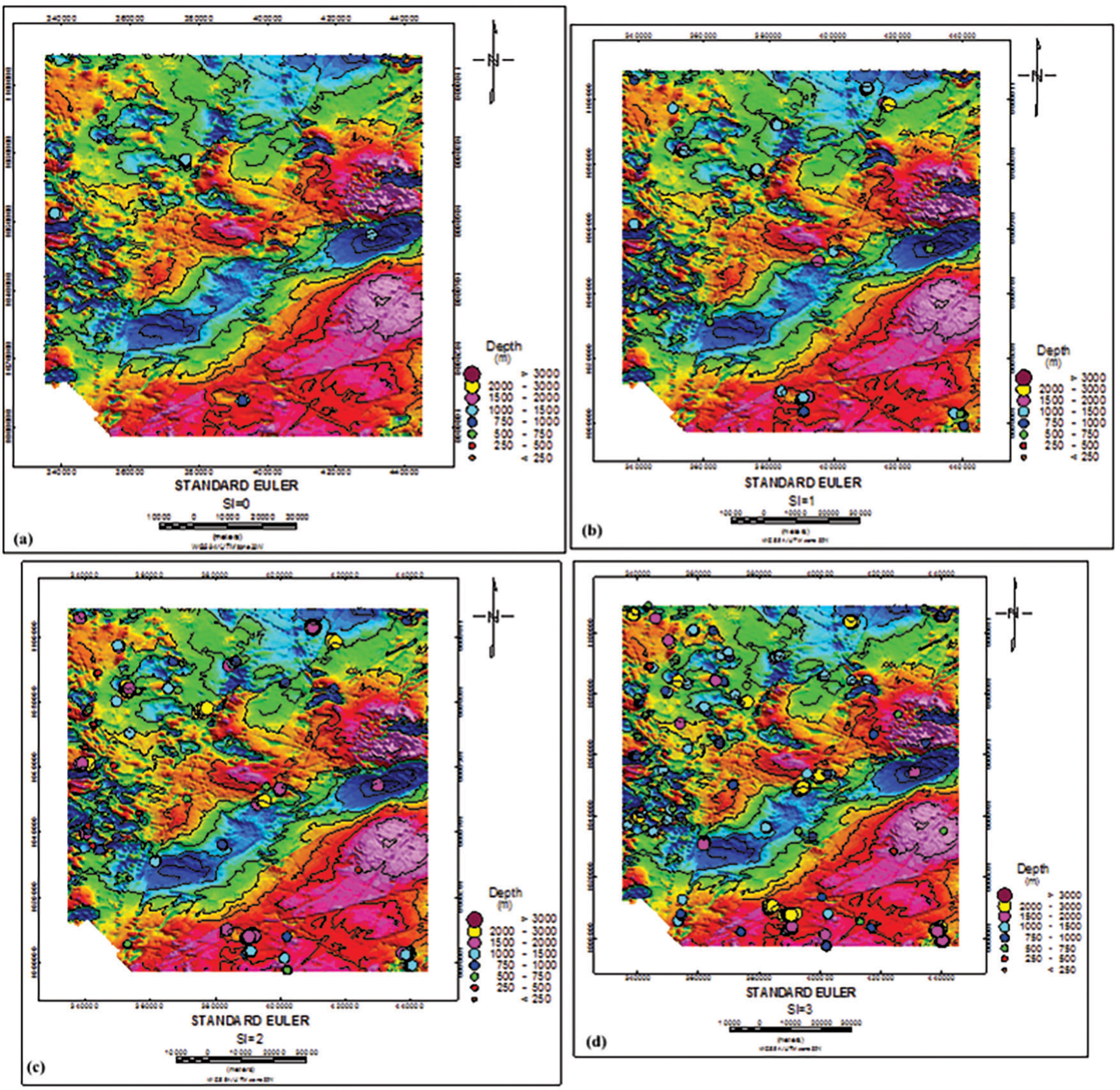
Figure 13:
3D Euler deconvolution depth solutions of the study area: (a) structural index = 0, (b) structural index = 1, (c) structural index = 2, (d) structural index = 3.