


Figure 1
Levels of accuracy of locating underground utility networks according to BSI (2014)
Table 1
Classification of quality levels (source: BSI (2014))
| Type of study | QL | Post-processing | Location accuracy | Additional data | ||
|---|---|---|---|---|---|---|
| Horizontal1 | Vertical2 | |||||
| D | Desktop utility records search | QL-D | - | Undefined | Undefined | - |
| C | Site reconnaissance | QL-C | - | Undefined | Undefined | Location of underground utilities in relation to above-ground objects. |
| QL-B4 | No | Undefined | Undefined | A presumably existing object – it has not been detected despite the existing information. | ||
| B | Detection3 | QL-B3 | No | ± 0.5 m | Undefined | Horizontal position of the object detected using one of the applied geophysical techniques. |
| QL-B3P | Yes | |||||
| QL-B2 | No | ± 0.25 m or ± 40% of detected depth | ±40% of ± detected depth | Horizontal and vertical positions of the object detected using one of the applied geophysical techniques.4 | ||
| QL-B2P | Yes | |||||
| QL-B1 | No | ± 0.15 m or ± 15% of detected depth | ± 15% of detected depth | Horizontal and vertical positions of the object detected by several applied geophysical techniques.5 | ||
| QL-B1P | Yes | |||||
| A | Verification | QL-A | - | ± 0.05 m | ± 0.025 m | Horizontal and vertical positions of the upper and/or lower part of underground utilities. |
[i] 1 Horizontal location is to the centreline of the utility.
2 Vertical location is to the top of utility.
3 For detection, it is a requirement that a minimum of GPR and EML techniques are used.
4 Electronic depth readings using EML equipment are not normally sufficient to achieve a QL-B2 or higher.
5 Some utilities can only be detected by one of the existing detection techniques. As a consequence, such utilities cannot be classified as a QL-B1.
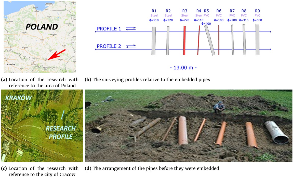
Figure 2
Draft of the location of the research and the arrangement of the pipes
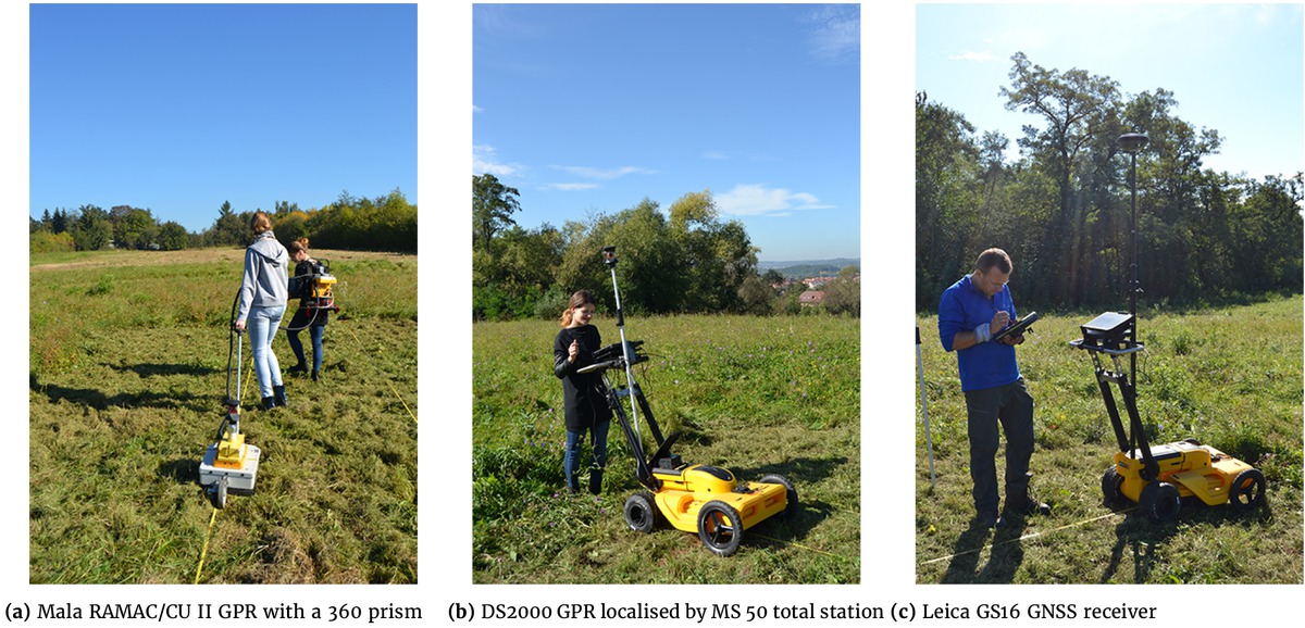
Figure 3
Surveying systems used
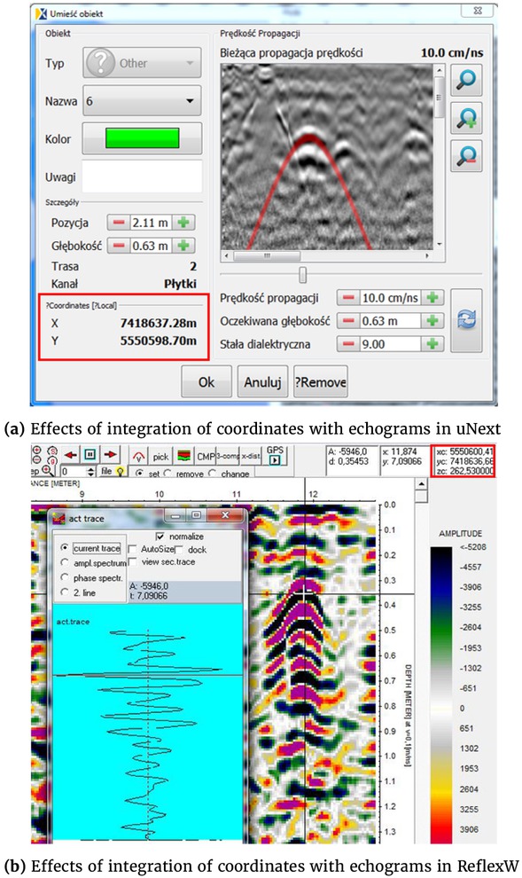
Figure 4
Effects of integration of coordinates with echograms
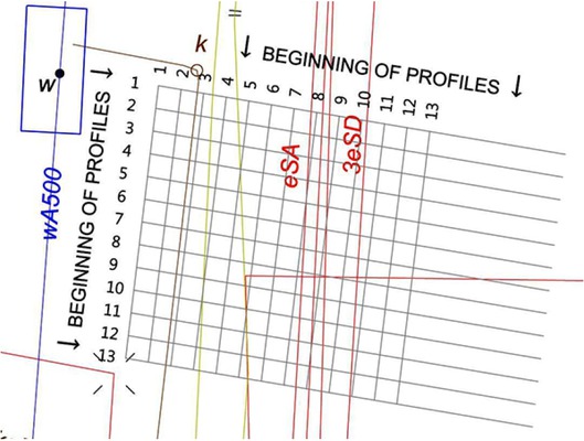
Figure 5
Arrangement of measurement profiles on available cartographic materials
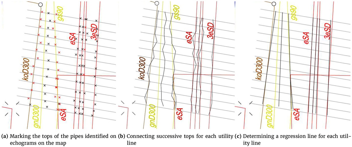
Figure 6
Scheme of detecting the profile of utilities based on the GPR method
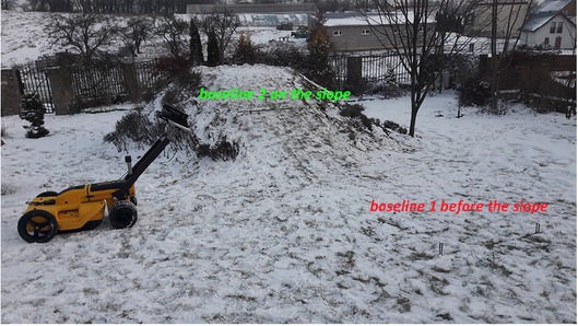
Figure 7
Location of the baselines of the supplementary measurement relative to the hill with a 45% slope
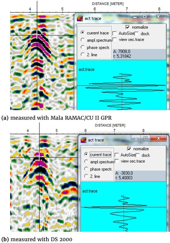
Figure 8
Polarisation of the wave reflected from the R1 pipe
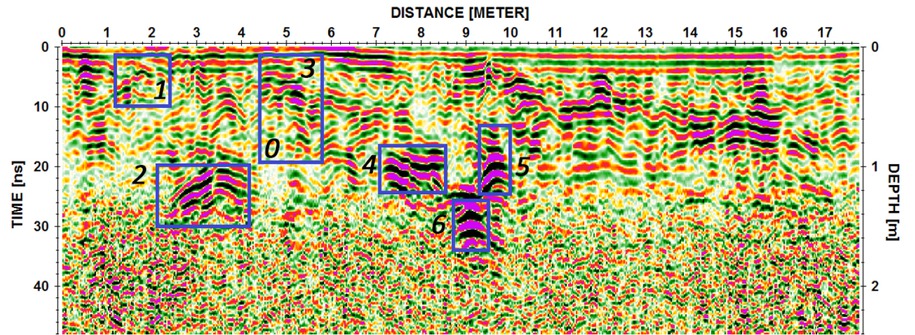
Figure 9
Classified echogram of the transverse trace – profile 12. Numbers of the areas marked on the echograms correspond to: 0 – eSA1; 1 – koD300; 2 – gnD300; 3 – gs90; 4 – eSA2, eSA3, eSA4; 5 – 3eSD; 6 – unidentified on cartographic materials utility line.
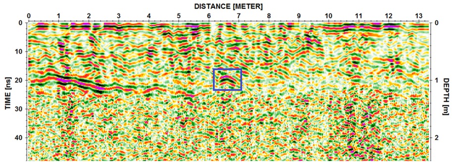
Figure 10
Echogram of the longitudinal trace – profile 10. The marked area of the occurrence of the eSA1 power line.
Table 2
Errors of fitting MNK regression lines [m]
| Method | gnD300 | gs90 | eSA1 | eSA2 | eSA3 | eSA4 | 3eSD |
|---|---|---|---|---|---|---|---|
| GPR-MS50 | 0.15 | 0.21 | 0.17 | 0.17 | 0.11 | 0.13 | 0.12 |
| Distance | 0.14 | 0.17 | 0.14 | 0.15 | 0.15 | 0.15 | 0.09 |
Table 3
Distances of regression lines relative to cartographic materials [m]
| GPR-MS50 method | gnD300 | gs90 | eSA1 | eSA2 | eSA3 | eSA4 | 3eSD |
|---|---|---|---|---|---|---|---|
| Min | 0.41 | -0.04 | -0.04 | -0.01 | -0.01 | -0.13 | -0.22 |
| Max | 0.53 | 0.09 | 0.24 | 0.05 | 0.03 | 0.03 | 0.08 |
| Mean | 0.47 | 0.02 | 0.10 | 0.02 | 0.01 | -0.05 | -0.06 |
| Distance method1 | gnD300 | gs90 | eSA1 | eSA2 | eSA3 | eSA4 | 3eSD |
| Min | 0.37 | -0.14 | -0.11 | -0.23 | -0.21 | -0.25 | -0.39 |
| Max | 0.46 | 0.09 | 0.16 | -0.11 | -0.11 | -0.16 | -0.10 |
| Mean | 0.42 | -0.04 | 0.02 | -0.17 | -0.16 | -0.20 | -0.24 |
[i] 1 Distance: profile from documentation – approximated profile [m]
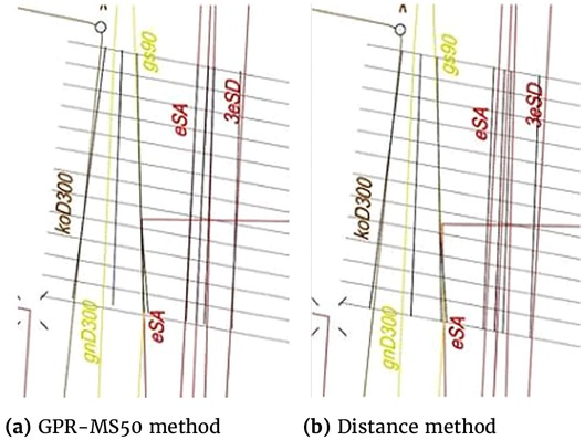
Figure 11
Obtained regression lines
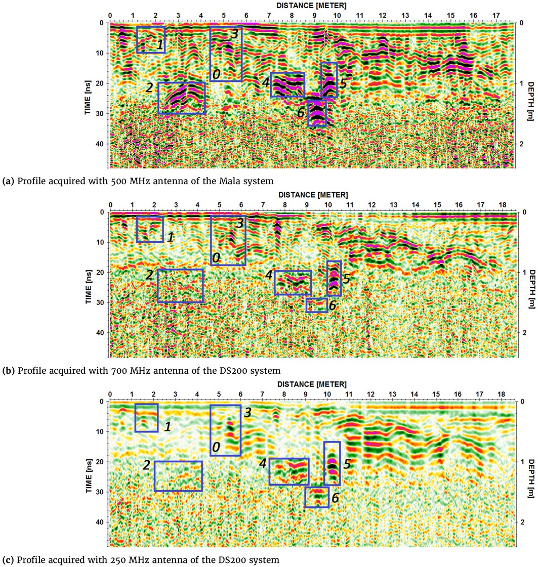
Figure 12
Echograms for the profile 12
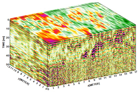
Figure 13
3D model created based on 2D echograms (B-scan)
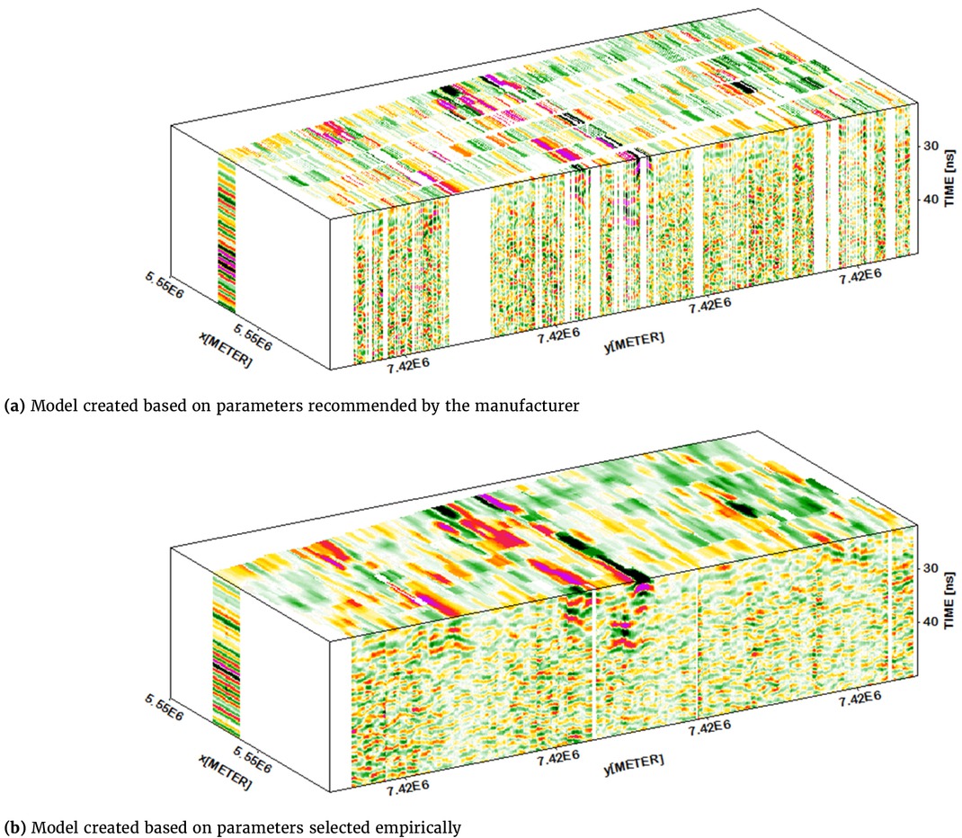
Figure 14
3D model with regard to georeference
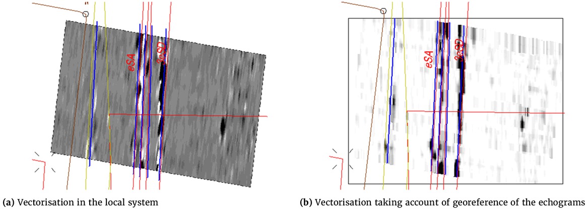
Figure 15
Vectorisation of the utility line axes based on the slice generated from the 3D model