

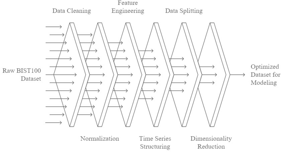
Fig. 1:
Data Preprocessing for Machine Learning
Tab. 1:
Characteristics of the dataset
| Variable | Description |
|---|---|
| Date | Date of observation |
| Open | Opening price on the given day |
| High | Highest price on the given day |
| Low | Lowest price on the given day |
| Close | Closing price on the given day |
| Simple Moving Average (SMA) | Average of closing prices over a specified period |
| Weighted Moving Average (WMA) | Average of closing prices over a specified period, weighted by recent prices |
| Momentum (MOM) | Rate of change of the closing price over a specified period |
| Stochastic %K (STCK) | Current closing price relative to the range over a recent period |
| Stochastic %D (STCD) | Moving average of the Stochastic %K |
| Relative Strength Index (RSI) | Measures the magnitude of recent price changes to evaluate overbought or oversold conditions |
| Moving Average Convergence Divergence (MACD) | Difference between the 12-day and 26-day exponential moving averages (EMAs) |
| Larry William’s %R (LWR) | Momentum indicator measuring overbought and oversold levels |
| Accumulation/Distribution Oscillator (ADO) | Indicator combining price and volume to show how much of a stock is being accumulated or distributed |
| Commodity Channel Index (CCI) | Measures the deviation of the price from its average over a specified period, indicating overbought or oversold conditions |
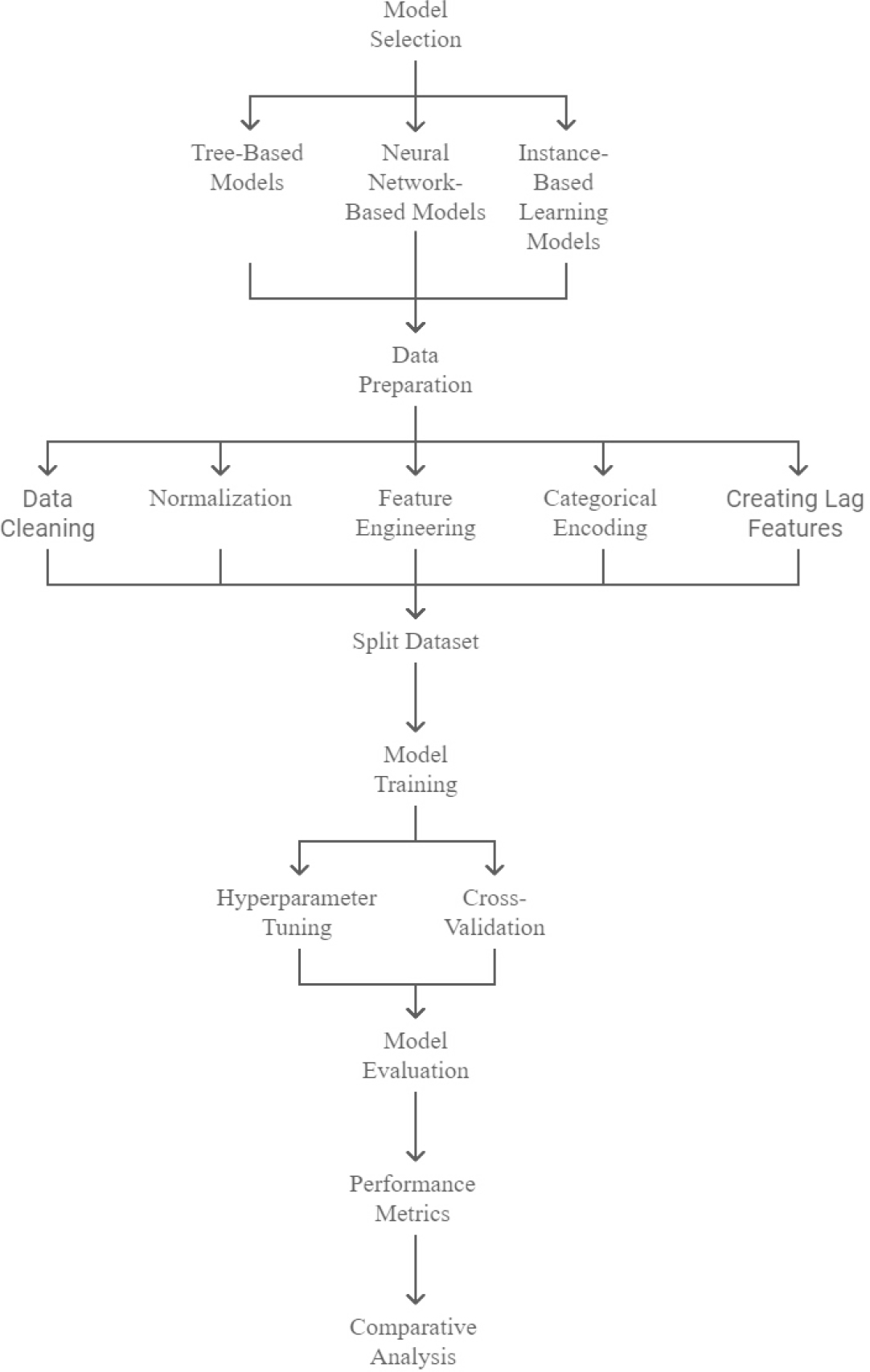
Fig. 2:
Experimental design of study
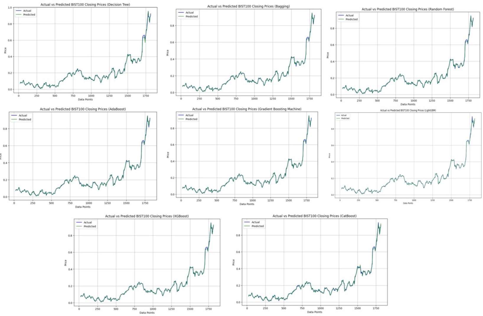
Fig. 3:
Tree-based models fitting results. Each subplot shows the predicted vs. actual closing prices for a specific Tree-Based Model (Decision Trees, Bagging, Random Forests, AdaBoost, GBM, LightGBM, XGBoost, CatBoost) applied to the BIST100 dataset. The blue line represents the actual closing prices, while the orange line represents the model’s predicted values. Closer alignment between the lines indicates higher predictive accuracy.
Tab. 2:
MSE, RMSE, MAE, MAPE and rRMSE values
| MSE | RMSE | MAE | MAPE | rRMSE | |
|---|---|---|---|---|---|
| Decision Trees | 3.258e–05 | 0.0057 | 0.0032 | 2.4591 | 0.0283 |
| Bagging | 1.671e–05 | 0.0041 | 0.0026 | 2.1876 | 0.0202 |
| Random Forests | 1.635e–05 | 0.0041 | 0.0024 | 1.9541 | 0.0201 |
| Adaboost | 2.272e–05 | 0.0047 | 0.0025 | 2.0166 | 0.0236 |
| GBM | 2.035e–05 | 0.0045 | 0.0023 | 1.6585 | 0.0223 |
| LightGBM | 2.739e–05 | 0.0052 | 0.0026 | 1.7510 | 0.0259 |
| XGBoost | 2.662e–05 | 0.0051 | 0.0025 | 1.7688 | 0.0256 |
| CatBoost | 3.129e–05 | 0.0055 | 0.0037 | 3.0035 | 0.0277 |
| ANN | 0.00042 | 0.0205 | 0.0151 | 13.6640 | 0.1019 |
| CNNs | 2.886e–05 | 0.0053 | 0.0039 | 4.1893 | 0.0266 |
| RNNs | 6.565e–05 | 0.0081 | 0.0060 | 5.6011 | 0.0402 |
| LSTMs | 0.0001 | 0.0106 | 0.0078 | 7.3147 | 0.0528 |
| KNN | 0.0001 | 0.0101 | 0.0071 | 7.0558 | 0.0501 |
| SVM | 1.592e–05 | 0.0039 | 0.0031 | 3.5148 | 0.0198 |
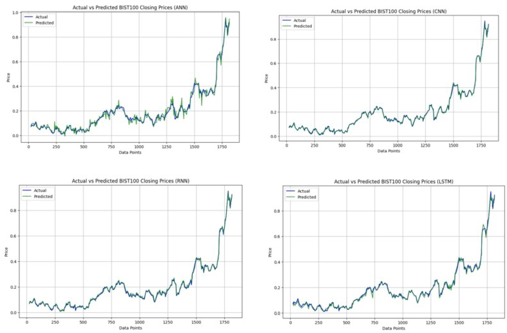
Fig. 4:
Neural Network-Based Models fitting results. This figure illustrates the predicted vs. actual financial performance for Neural Network-Based Models (ANN, CNN, RNN, LSTM) using the BIST100 dataset. Lower deviation from the diagonal line indicates better predictive accuracy.
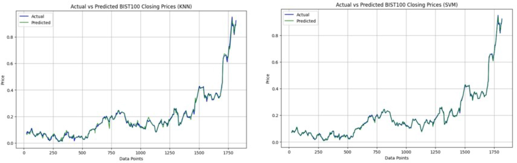
Fig. 5:
Instance-based Learning Models fitting results. This figure compares the predicted vs. actual financial performance for Instance-Based Learning Models (KNN, SVM) on the BIST100 dataset. Performance differences are reflected in the proximity of predictions to the actual values.