
TABLE 1.
Characteristics of the distribution of clinical data of patients among groups
| Clinical indicators | Training set (n = 265) | Validation set (n = 114) | External test set (n = 82) | Statistics | P value |
|---|---|---|---|---|---|
| Age (years) a | 43.0 (35.0–52.0) | 45.5 (35.3–54.0) | 45.0 (34.0–53.0) | 0.401 | 0.818 |
| Size (mm) a | 6.1 (4.7–7.8) | 5.6 (4.2–7.0) | 6.0 (4.6–7.3) | 4.090 | 0.129 |
| Aspect ratio a | 1.1 (0.9–1.3) | 1.0 (0.9–1.2) | 1.1 (0.9–1.3) | 3.547 | 0.170 |
| Sex | 1.493 | 0.474 | |||
| Male | 69 (26.0) | 24 (21.1) b | 23 (28.1) b | ||
| Female | 196 (74.0) | 90 (79.0) | 59 (72.0) | ||
| Location | 15.632 | 0.016 | |||
| Upper segment | 33 (12.5) | 15 (13.2) | 22 (26.8) b | ||
| Middle segment | 146 (55.1) | 58 (50.9) | 38 (46.3) | ||
| Lower segment | 57 (21.5) | 29 (25.4) | 20 (24.4) | ||
| Isthmus | 29 (10.9) | 12 (10.5) | 2 (2.4) | ||
| ETE | 4.733 | 0.094 | |||
| Absence | 226 (85.3) | 102 (89.5) | 77 (93.9) | ||
| Presence | 39 (14.7) | 12 (10.5) | 5 (6.1) | ||
| Echogenicity | 4.110 | 0.391 | |||
| Hyperechoic/isoechoic | 11 (4.2) | 8 (7.0) | 5 (6.1)b | ||
| Hypoechoic | 200 (75.5) | 75 (65.8) | 59 (72.0) | ||
| Markedly | |||||
| Hypoechoic | 54 (20.3) | 31 (27.2) | 18 (22.0) | ||
| Margin | 2.449 | 0.294 | |||
| Clear | 113 (42.6) | 53 (46.5) | 29 (35.4) | ||
| Unclear | 152 (57.4) | 61 (53.5) | 53 (64.6) | ||
| Shape | 5.242 | 0.073 | |||
| Regular | 115 (43.4) | 47 (41.2) | 24 (29.3) | ||
| Irregular | 150 (56.6) | 67 (58.8) | 58 (70.7) | ||
| Vascularity | 5.642 | 0.465 | |||
| Type I | 95 (35.9) | 38 (33.3) | 24 (29.3) | ||
| Type II | 21 (7.9) | 9 (7.9) | 12 (14.6) | ||
| Type III | 140 (52.8) | 63 (55.3) | 41 (50.0) | ||
| Type IV | 9 (3.4) | 4 (3.5) | 5 (6.1) | ||
| Calcification Absence | 123 (46.4) b | 58 (50.9) | 41 (50.0) | 2.902 | 0.821 |
| Microcalcification | 100 (37.7) | 38 (33.3) | 25 (30.5) | ||
| Coarse type | 25 (9.4) | 13 (11.4) | 10 (12.2) | ||
| Mixed type | 17 (6.4) | 5 (4.4) | 6 (7.3) | ||
| CC | 0.212 | 0.900 | |||
| Absence | 97 (36.6) | 41 (36.0) | 32 (39.0) | ||
| Presence | 168 (63.4) | 73 (64.0) | 50 (61.0) | ||
| DC | 0.496 | 0.780 | |||
| Absence | 186 (70.2) | 83 (72.8) | 56 (68.3) | ||
| Presence | 79 (29.8) | 31 (27.2) | 26 (31.7) | ||
1 Except for the special markings, the numbers in the table represent the number of patients, and the numbers in parentheses represent the percentage of the number of patients within the group.
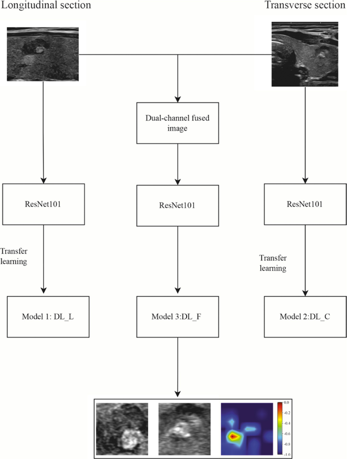
FIGURE 1.
Flowchart depicting the construction of the dual-channel deep learning model. The model comprises two components, Model 1 and Model 2, which are built using ultrasonic images from the longitudinal and transverse sections of the thyroid tumor, respectively. These images are then fused to create dual-channel images. The ResNet101 architecture is employed to train the fused model, referred to as DL_F (Model 3).
DL_C = cross-sectional deep learning model; DL_F = deep learning model using dual-channel fused images; DL_L = longitudinal deep learning model
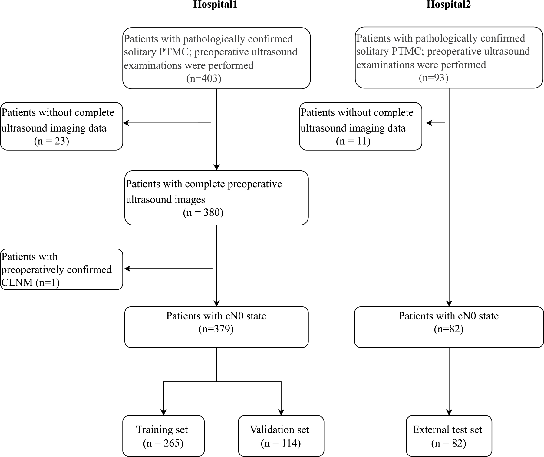
FIGURE 2.
Flowchart illustrating the patient enrollment process.
PTC = papillary thyroid carcinoma; PTMC = papillary thyroid microcarcinoma; CLNM = cervical lymph node metastasis
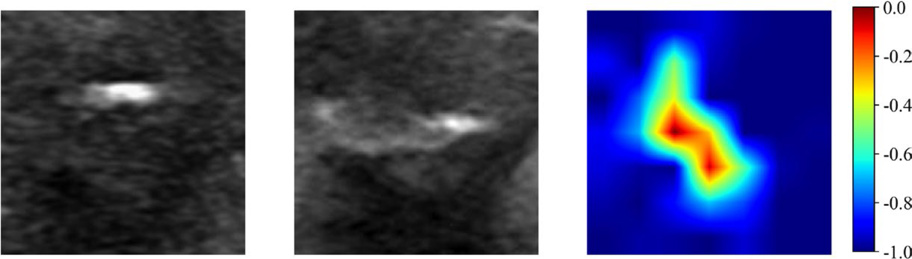
FIGURE 3.
Gradient-weighted Class Activation Mapping images predicted by the dual-channel deep learning model. The left image represents the minimum bounding rectangle containing the largest section of the tumor on the longitudinal section. The middle image represents the minimum bounding rectangle containing the largest section of the tumor on the transverse section. The right image represents the Gradient-weighted Class Activation Mapping image.
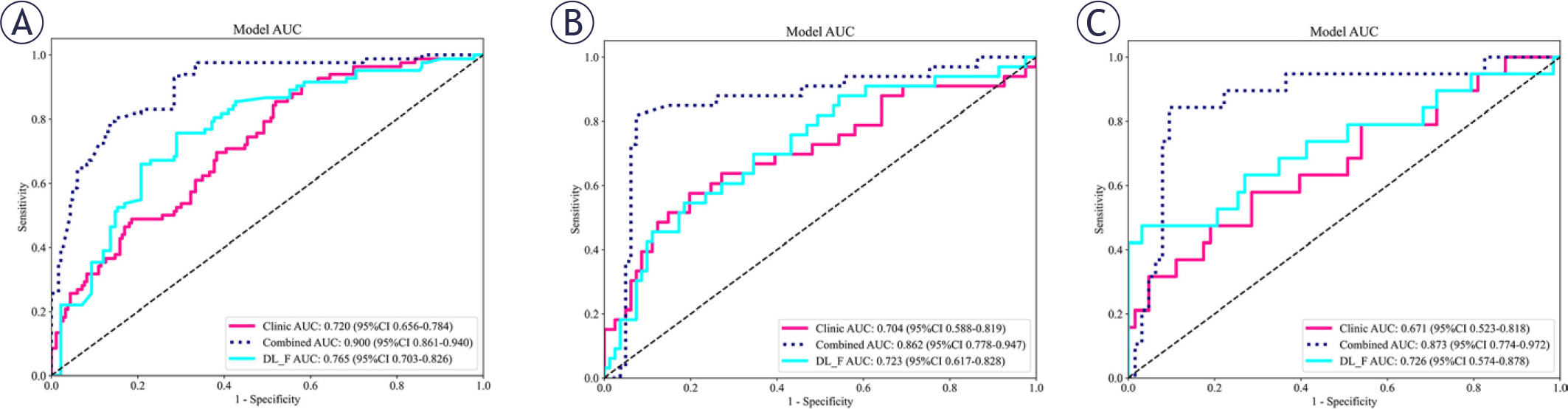
FIGURE 4.
The AUC values of the combined model. Compared with the clinical model and the dual-channel model, the combined model has higher AUC values on the training set (A), the validation set (B), and the external test set (C).
AUC = area under the receiver operating characteristic curve; CI = confidence interval; LightGBM = Light Gradient Boosting Machin; LR = logistic regression
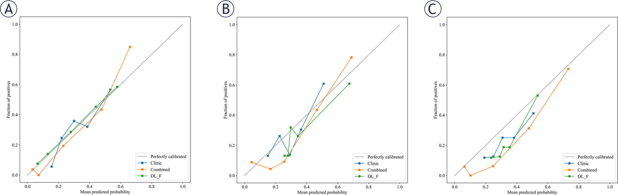
FIGURE 5.
Calibration curves of different models. (A) Calibration curves of the combined model, dual-channel model and the clinical model in training dataset; (B) Calibration curves in the validation dataset; (C) Calibration curves in the external test set.
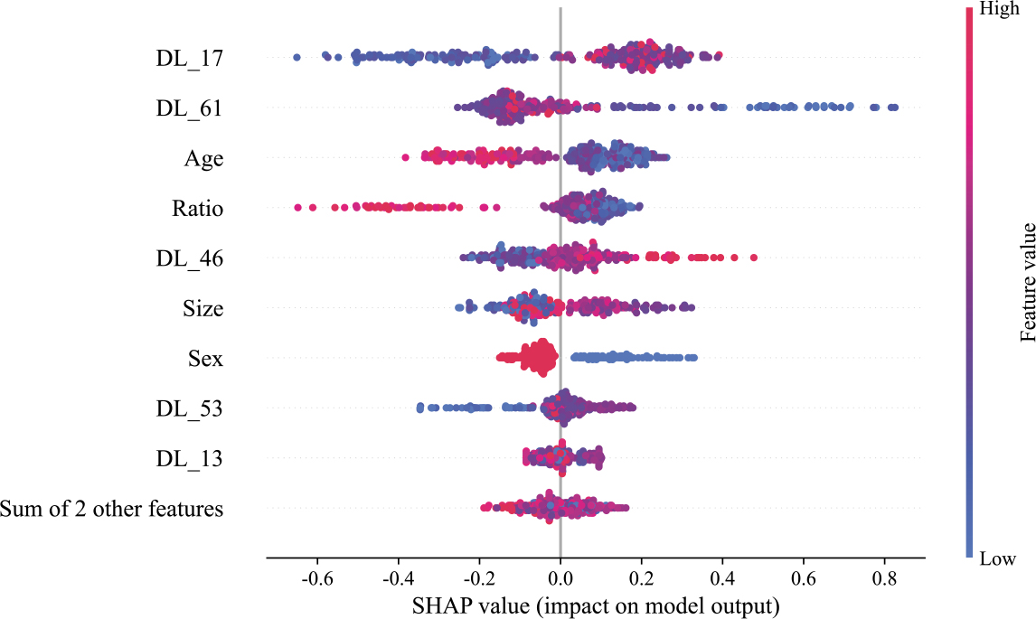
FIGURE 6.
Contributions of individual features in the combined model. The summary plot displays the distribution of SHAP values for each feature across all predictions in the training cohort, providing a comprehensive overview of feature importance and their respective impacts.
SHAP = SHapley Additive exPlanations