
Table 1
Studies on NR, human capital, energy consumption, and the EF.
| Author(s) | Time period | Methodology | Variables considered | Country(ies) | Key finding(s) |
|---|---|---|---|---|---|
| Nathaniel (2021) | 1990–2016 | AMG | NRR, GDP, HC, EF | ASEAN bloc | NRR does not hurt environment in Thailand and Laos PDR. Bidirectional causality exists between HC and GDP, and between NRR and GDP. |
| Ulucak et al. (2020) | 1995–2016 | DOLS, FMOLS. | EF, GDP, NRR, URB, REN | BRICS | REN, URB, and NRR decrease EF. GDP enhances environmental degradation. |
| Ahmed et al. (2020a) | 1970–2016 | ARDL | NRR, HC, GDP, URB, EF | China | URB, NRR, and GDP drive EF in China. |
| Ahmed et al. (2020b) | 1971–2014 | CUP-FM, CUP-BC. | FDI, GDP, NRE, URB, HC, EF | G7 countries. | GDP, NRE, and URB increase EF, while HC and FDI reduce it. |
| Nathaniel (2020) | 1971–2014 | ARDL | GDP, NRE, URB, TRD, EF | Indonesia | NRE, GDP, and URB increase EF in Indonesia. |
| Baloch et al. (2019a) | 1990–2016 | Driscoll-Kraay panel regression | FDI, GDP, FDV, NRE, URB, EF | 59 Belt and Road countries. | FDV, FDI, NRE and URB have negative influence on environment. |
| Hassan et al. (2019a) | 1971–2014 | ARDL | NRR, GDP, BIO, GDP2 EF | Pakistan | Long-run causality exists between BIO and EF. NRR has positive impact on EF. |
| Hassan et al. (2019b) | 1971–2014 | ARDL | HC, GDP, BIO, EF | Pakistan | BIO increases EF. GDP declines EF by 0.60%. HC exerts negative effect on EF. GDP Granger causes EF. |
| Dogan et al. (2019) | 1971–2013 | ARDL | Fossil fuel energy, URB, Export, FDV, REN, EF | Mexico, Indonesia, Nigeria, and Turkey. | URB is chief cause of environmental degradation. |
| Nathaniel et al. (2020c) | 1990–2016 | AMG | REN, NRE, URB, EF, FDV, GDP | MENA | FDV, GDP, NRE, and URB increase EF in MENA. One-way causality flows from NRE and URB to EF. |
| Nathaniel et al. (2020d) | 1980–2016 | Panel Quantile Regression | FDI, EF, NRE, URB, GDP, carbon footprint, CO2 emissions | Coastal Mediterranean countries | NRE degrades environment. Effects of GDP and URB on environment were mixed for different indicators. |
| Ulucak et al. (2020) | 1992–2016 | FMOLS, DOLS. | NRR, URB, REN, GDP, GDP2, EF | BRICS | EKC is validated in individual BRICS countries. NRR, URB, and REN reduce EF. |
| Destek, Sinha (2020) | 1980–2014 | MG. FMOLS-MG, DOLS-MG. | GDP, GDP2, EF, REN, TRD, NRE | 24 OECD countries. | EKC hypothesis does not hold. REN reduces EF. |
| Wang, Dong (2019) | 1990–2014 | AMG | REN, URB, GDP, GDP2, EF, NRE | 14 SSA countries. | Feedback causality runs among NRE, URB, GDP, and EF. NRE, GDP, and URB exert positive effects on EF. |
| Sharma et al. (2020) | 1990–2015 | Panel ARDL | REN, URB, POP, FOR, NRE, GDP, EF | Asia | URB, GDP, NRE, FOR, and POP drive EF. REN restores environmental quality. |
| Ansari et al. (2020) | 1991–2017 | PMG | EF, URB, Material footprint, GDP, GLO, NRE | 37 Asian countries | URB and GLO increase EF. GDP and NRE also increase EF. |
| Sharif et al. (2020) | 1965Q1–2017Q4 | Quantile ARDL | NRE, EF, REN, GDP | Turkey | Feedback causality exists among listed variables; RE, GDP, NRE, and EF. |
| Altıntaş, Kassouri (2020) | 1990–2014 | CCEMG, IFE. | CO2 emissions, EF, RE, GDP, NRE | Europe | RE is environmentally friendly. NRE exerts positive impact on EF. |
| Baz et al. (2020) | 1971–2014 | NARDL | GDP, NRE Capital, EF | Pakistan | EF Granger causes NRE. GDP does not cause EF. |
| Aziz et al. (2020) | 1990–2018 | QARDL | GDP, EF, FOR, RE | Pakistan | FOR and REN minimise EF. GDP increases EF thereby encouraging environmental degradation. |
[i] Note: ARDL – autoregressive distributed lag model; QARDL: BRICS – Brazil, Russia, India, China and South Africa; BIO – biocapacity; CUP-FM – continuously updated fully modified; CUP-BC – continuously updated bias-corrected; DOLS – dynamic ordinary least squares; EF – ecological footprint; EKC – Environmental Kuznets Curve; FDI – Foreign Direct Investment; FOR – forest; FMOLS – fully modified ordinary least squares; FDV – Financial Development; GLO – globalisation; HC – human capital; IFE – interactive fixed effects; MG – mean group; MENA – Middle East and North Africa; NR – natural resources; NRE – non-renewable energy; NARDL – non-linear ARDL; POP – population; REN – renewable energy; SSA – Sub-Saharan Africa; TRD – trade openness; TRD – trade; Quantile ARDL; URB – urbanisation.
[ii] Source: own compilation.
Table 2
Measurement and source of data.
| S/N | Indicator name | Measurement | Source |
|---|---|---|---|
| 1 | Urbanisation | Urban population (% of total population) | WDI (2019) |
| 2 | Natural resources | Total natural resource rent (% of GDP) | ✓ |
| 3 | GDP per capita | In constant 2010 USD | ✓ |
| 4 | Interaction term | (Human capital × Urbanisation) | ✓ |
| 5 | GDP per capita2 | In constant 2010 USD | ✓ |
| 6 | Ecological footprint | Global hectares per capita | GFN (2019) |
| 7 | Human capital | Human capital index | Penn World Table |
[i] GFN – global footprint network; WDI – World Development Indicator.
[ii] Source: own compilation.
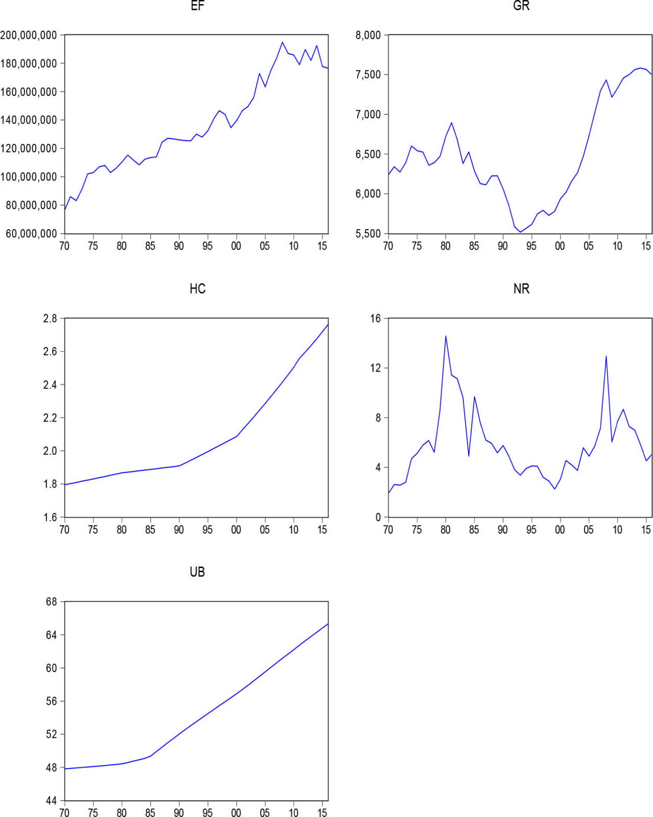
Fig. 1
Plots of the series. EF – ecological footprint; HC – human capital; NR – natural resources; UB – urbanisation.
Source: own compilation.
Table 3
Descriptive statistics.
| EF | GR | GR | NR | HC | UB | IN | |
|---|---|---|---|---|---|---|---|
| Mean | 1.070 | 8.772 | 14.51 | 1.657 | 0.727 | 3.991 | 0.549 |
| Max. | 3.930 | 8.933 | 15.05 | 2.678 | 1.016 | 4.179 | 0.801 |
| Min. | 1.100 | 8.615 | 14.00 | 0.650 | 0.584 | 3.867 | 0.426 |
| Std. D | 0.245 | 0.093 | 0.309 | 0.460 | 0.131 | 0.104 | 0.114 |
| Skewness | −0.117 | 0.265 | 0.281 | 0.062 | 0.862 | 0.311 | 0.836 |
| Kurtosis | 2.198 | 2.126 | 2.128 | 2.707 | 2.384 | 1.669 | 2.350 |
| Prob. | 0.505 | 0.359 | 0.348 | 0.905 | 0.037 | 0.120 | 0.042 |
[i] EF – ecological footprint; HC – human capital; NR – natural resources; UB – urbanisation; GR – economic growth; IN – interaction between HC and UB.
[ii] Source: author's computation.
Table 4
Results of the DF-GLS and NG-Perron unit root tests.
| Variables | DF-GLS | NG-Perron | ||||
|---|---|---|---|---|---|---|
| At level | Difference | At level | Difference | |||
| t-statistic | t-statistic | t-statistic | MSB 5% | t-statistic | MSB 5% | |
| EF | 0.091 | −6.811*** | 0.829 | 0.233 | 0.148** | 0.233 |
| GR | −0.846 | −4.228*** | 0.346 | 0.233 | 0.162** | 0.233 |
| HC | −0.318*** | −0.208 | 0.244** | 0.233 | 0.559 | 0.233 |
| NR | −2.426 | −8.647*** | 0.234 | 0.233 | 0.154*** | 0.233 |
| UB | −1.702*** | −0.797 | 0.143** | 0.233 | 0.519 | 0.233 |
| IN | −0.528*** | −0.474 | 0.228** | 0.233 | 0.551 | 0.233 |
| GR2 | −0.920 | −4.152*** | 0.338 | 0.233 | 0.164*** | 0.233 |
Table 5
ZA unit root results.
Table 6
Bounds test results.
| Models | Lower bound | Upper bound | Significance level |
|---|---|---|---|
| Model 1 | |||
| Fc (lngr, lnnr, lnhc, lnub). F = 8.3425 | 2.25 2.86 3.69 | 3.59 3.76 4.46 | 10% 5% 1% |
| Model 2 | |||
| Fc (lngr, lnnr, lnhc, lnub, lnin). F = 7.6069 | 1.81 2.14 2.82 | 2.93 3.34 4.21 | 10% 5% 1% |
| Model 3 | |||
| Fc (lngr, lnnr, lnhc, lnub, lngr2). F = 8.5647 | 2.29 2.71 3.46 | 3.38 4.56 4.76 | 10% 5% 1% |
[i] Source: author's computation.
Table 7
BH test results.
| Estimated models | EG − JOH | EG − JOH − BO − BDM | Cointegration |
|---|---|---|---|
| lnEF = f(lnGR,lnNR,lnHC,lnUB) | 14.651 | 38.854 | Yes |
| lnEF = f(lnGR,lnNR,lnHC,lnUB,lnIN) | 21.361 | 44.537 | Yes |
| lnEF = f(lnGR,lnNR,lnHC,lnUB,lnGR2) | 15.101 | 36.342 | Yes |
| 5% critical value (for Model 1) | 10.576 | 20.143 | |
| 5% critical value (for Models 2 and 3) | 10.419 | 19.888 |
[i] Note: ** represents 0.05% significance level.
[ii] EF – ecological footprint; HC – human capital; NR – natural resources; UB – urbanisation.
[iii] Source: author's computation.
Table 8
ARDL results.
| Long-run results | |||
|---|---|---|---|
| Variables | Model 1 | Model 2 | Model 3 |
| Constant | 4.162** | 4.432** | 2.465 |
| (2.478) | (3.441) | (1.047) | |
| GR (log) | 0.032** | 0.546*** | 0.129*** |
| (2.675) | (4.567) | (3.657) | |
| HC (log) | −0.044** | −0.146** | −0.198*** |
| (−2.987) | (−2.286) | (−3.892) | |
| NR (log) | 0.275*** | 0.297*** | 0.140*** |
| (2.979) | (3.486) | (3.287) | |
| UB (log) | 0.450*** | 0.228*** | 0.052*** |
| (7.657) | (6.836) | (6.679) | |
| IN (log) | – | −0.231*** | – |
| – | (−4.675) | – | |
| GR2 (log) | – | – | −0.056*** |
| – | – | (−7.546) | |
| Short-run results | |||
|---|---|---|---|
| Variables | Model 1 | Model 2 | Model 3 |
| EF(−1) (log) | −0.298*** | −0.672*** | −0.098*** |
| (−4.564) | (−6.978) | (−7.619) | |
| Dlog(HC) | −1.324 | −0.174** | −1.534 |
| (−0.246) | (−2.167) | (−0.678) | |
| Dlog(HC(−1)) | 1.349 | −0.437 | 1.872 |
| (0.392) | (−1.443) | (0.954) | |
| Dlog(NR) | 0.032*** | 0.060*** | 0.007* |
| (5.923) | (5.823) | (1.878) | |
| Dlog(NR(−2) | 0.062 | – | 0.567 |
| (1.409) | – | (1.765) | |
| Dlog(UB) | 0.629*** | 0.672*** | 0.050*** |
| (6.867) | (7.562) | (6.985) | |
| Dlog(GR) | 0.045*** | 0.045*** | 1.546 |
| (4.670) | (3.967) | (0.845) | |
| CointEq(−1)* | −0.986*** | −0.876*** | −0.156*** |
| (−8.719) | (−7.491) | (−6.821) | |
| Diagnostic tests | |||
| R-squared | 0.767 | 0.627 | 0.843 |
| χ2 Jarque-Bera | 0.867 | 0.965 | 0.825 |
| χ2 LM test | 0.629 | 0.564 | 0.725 |
| χ2 Ramsey | 0.185 | 0.487 | 0.627 |
| χ2 Breusch-Pagan-Godfrey | 0.489 | 0.646 | 0.342 |
[i] Note: ***, ** and * represent statistical significance at the 1%, 5% and 10% levels of significance respectively; t-statistics are in parentheses.
[ii] ARDL – autoregressive distributed lag; EF – ecological footprint; HC – human capital; NR – natural resources; UB – urbanisation.
[iii] Source: author's computation.
Table 9
Robustness check.
| Variables | FMOLS | DOLS | CCR |
|---|---|---|---|
| GR (log) | 0.056** | 0.202** | 0.326*** |
| (2.276) | (2.581) | (4.768) | |
| HC (log) | −0.064*** | −1.667*** | −0.621*** |
| (−5.835) | (−9.673) | (−8.289) | |
| NR (log) | 0.024*** | 0.241*** | 1.046*** |
| (3.768) | (4.573) | (9.231) | |
| UB (log) | 0.348*** | 0.271*** | 0.2286*** |
| (3.987) | (9.482) | (7.271) |
[i] Note: *** and ** represent statistical significance at the 1% and 5% levels respectively; t-statistics are in parentheses.
[ii] CCR – canonical regression; DOLS – dynamic ordinary least squares; FMOLS – fully modified ordinary least squares; HC – human capital; NR – natural resources; UB – urbanisation.
[iii] Source: author's computation.
Table 10
Toda-Yamamoto test results.
| Null Hypotheses | MWALD Stat. | Probability | Causality |
|---|---|---|---|
| GR→EF | 6.015 | 0.021 | Yes |
| HC→EF | 5.892 | 0.044 | Yes |
| NR→EF | 4.042 | 0.120 | No |
| UB→EF | 8.763 | 0.007 | Yes |
| EF→GR | 7.382 | 0.035 | Yes |
| HC→GR | 9.702 | 0.031 | Yes |
| NR→GR | 5.819 | 0.042 | Yes |
| UB→GR | 8.281 | 0.018 | Yes |
| EF→HC | 1.745 | 0.650 | No |
| GR→HC | 0.619 | 0.723 | No |
| NR→HC | 1.891 | 0.634 | No |
| UB→HC | 2.817 | 0.380 | No |
| EF→NR | 0.483 | 0.066 | Yes |
| GR→NR | 0.581 | 0.001 | Yes |
| HC→NR | 1.291 | 0.035 | Yes |
| UB→NR | 9.382 | 0.491 | No |
| EF→UB | 0.173 | 0.849 | No |
| GR→UB | 0.481 | 0.341 | No |
| HC→UB | 1.461 | 0.635 | No |
| NR→UB | 9.903 | 0.045 | Yes |
[i] Note: All the variables are logged.
[ii] EF – ecological footprint; HC – human capital; NR – natural resources; UB – urbanisation.
[iii] Source: author's computation.
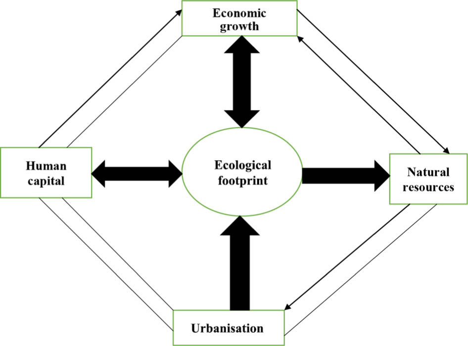
Fig. 2
Causality relationship schema.
EF – ecological footprint; HC – human capital; NR – natural resources; UB – urbanisation.
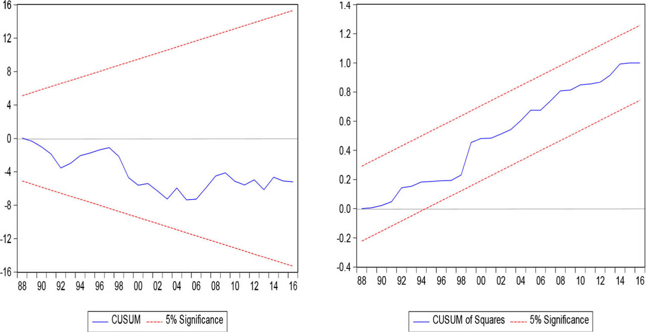
Fig. 3
Cusum and Cusumsq plots for Model 1.
Source: own compilation.
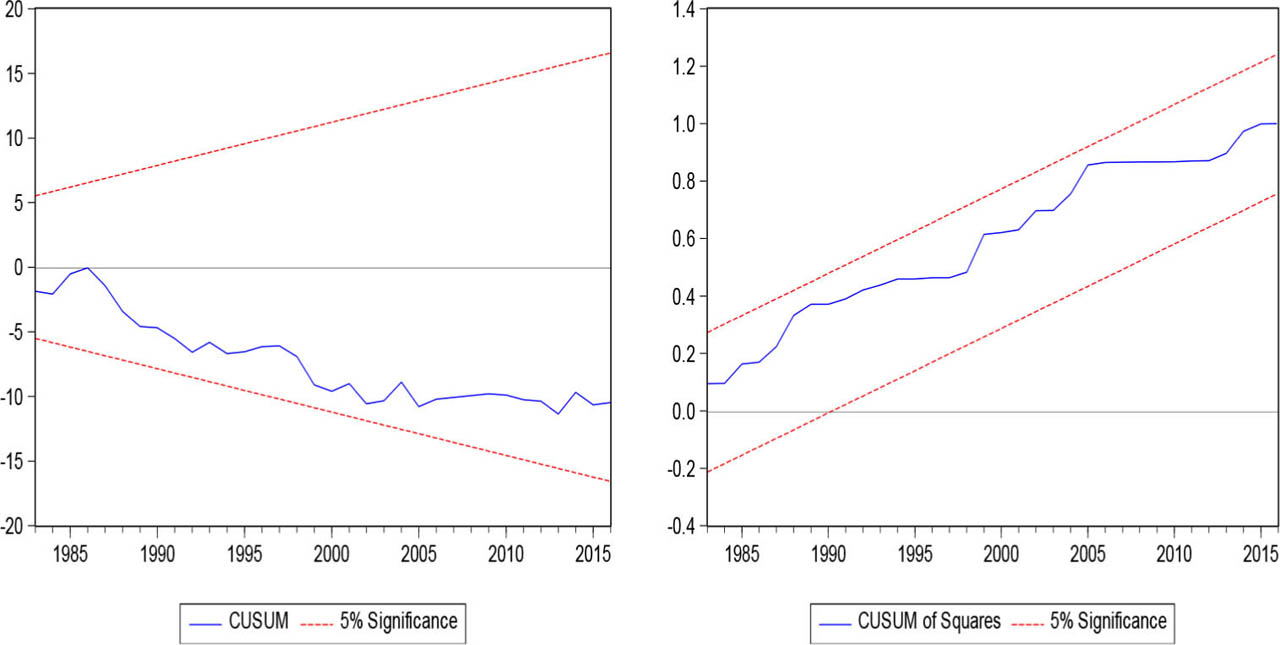
Fig. 4
Cusum and Cusumsq plots for Model 2.
Source: own compilation.
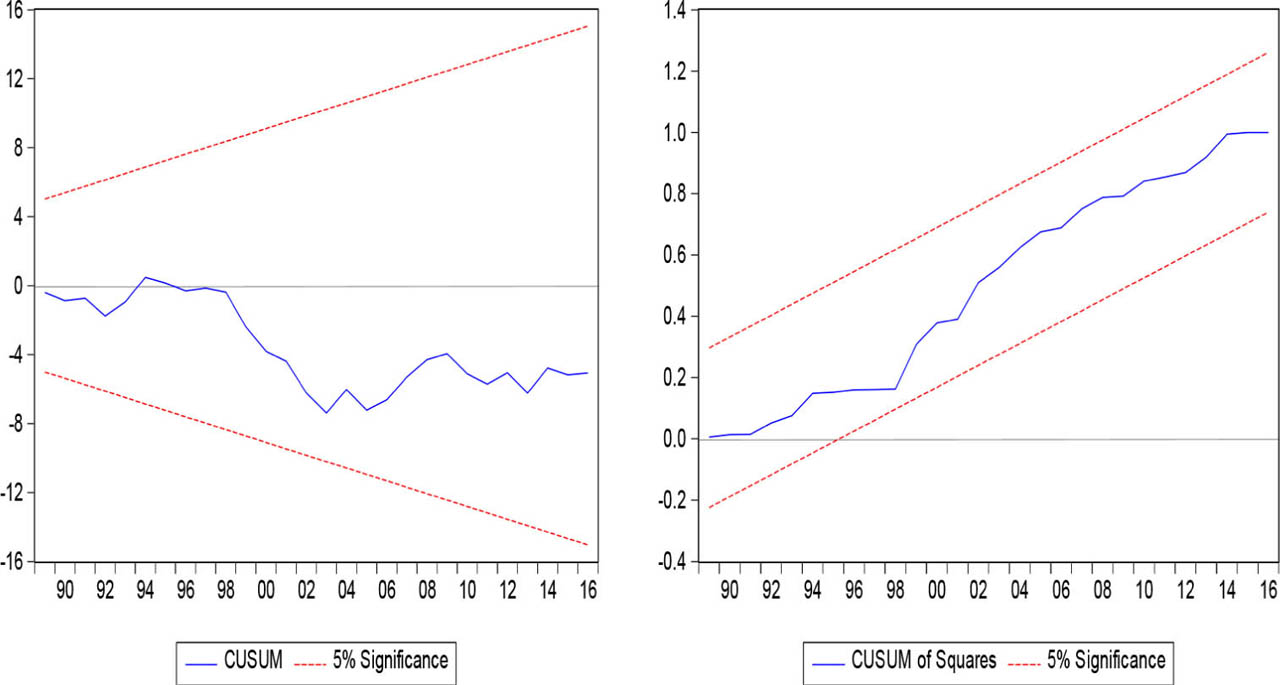
Fig. 5
Cusum and Cusumsq plots for Model 3.
Source: own compilation.