
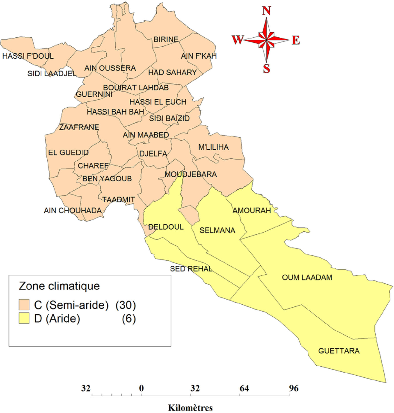
Fig. 1
Climate zone in the department of Djelfa. Based on DTR 3.2: 2004.
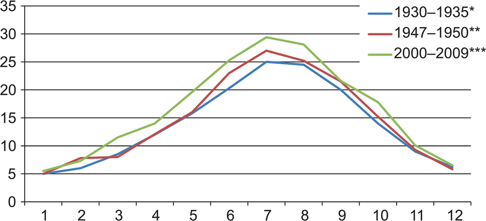
Fig. 2
Temperature variation between 1930 and 2004.
Table 1
Mean values, standard deviation and test of normality of the variables.
| With log10 transformation | ||||||
|---|---|---|---|---|---|---|
| Variables (2013) | Mean | Std deviation | Skewness | Kurtosis | Skewness | Kurtosis |
| gas subscribers | 3126.86 | 7523.27 | 4.35 | 21.32 | 0.80 | 0.13 |
| gas consumption (Kth) | 80545.56 | 210208.39 | 4.84 | 25.86 | 0.72 | 0.11 |
| electricity subscribers | 3968.75 | 8209.25 | 4.13 | 19.38 | 0.74 | 0.56 |
| electricity consumption (mwh) | 10139.75 | 21255.03 | 4.18 | 19.66 | 0.51 | 0.56 |
| number of population | 35667.14 | 64194.61 | 4.51 | 22.92 | 0.32 | 1.77 |
| number of housing | 6256.29 | 9888.58 | 4.03 | 18.07 | 0.91 | 0.59 |
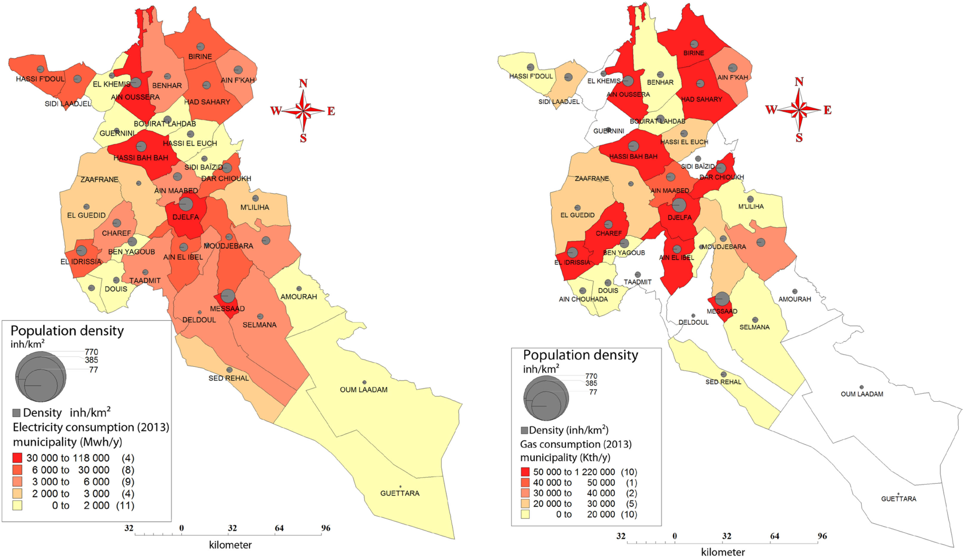
Fig. 3
Consumption of (a) electricity and (b) gas by residential buildings in 2013.
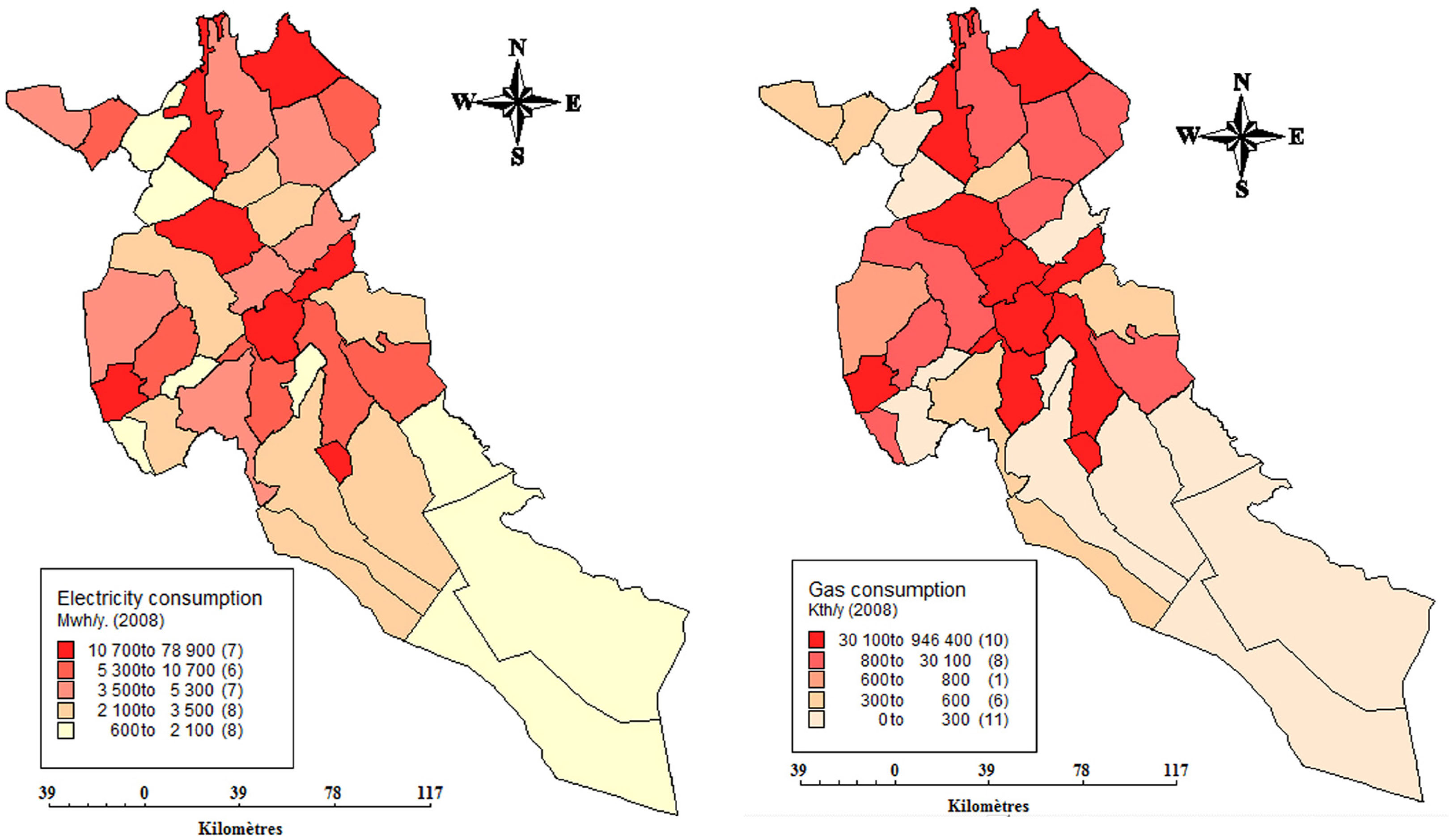
Fig. 4
Gas and electricity consumption in 2008 per municipality.
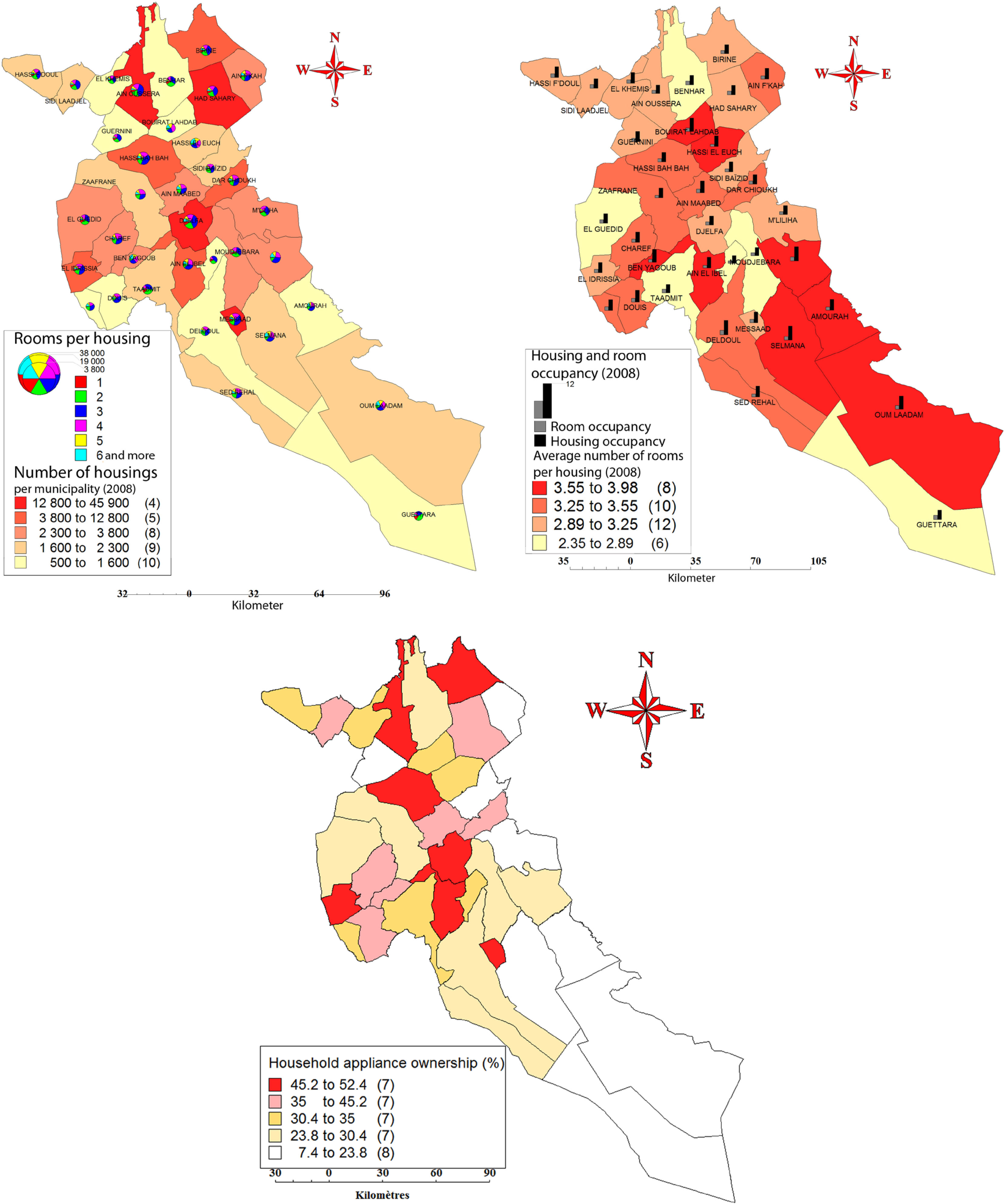
Fig. 5
(a) housing number and size, (b) household size, room occupancy and average number of rooms per housing, (c) appliance ownership (TV, cooker, washing machine, refrigerator and air conditioner).
Table 2
Summary of the gas and electricity model.
| Electricity model summary (R2=0.937) | Gas model summary (R2= 0.986) | ||||||||
|---|---|---|---|---|---|---|---|---|---|
| model | unstandardised coefficients | standardised coefficients | Sig. | model | unstandardised coefficients | standardised coefficients | Sig. | ||
| B | Std. error | Beta | B | Std. error | Beta | ||||
| (constant) | 0.927 | 0.268 | 0.002 | (constant) | 1.635 | .163 | .000 | ||
| log10_electricity subscribers | 1.239 | 0.097 | 1.178 | 0.000 | log10_gas_subscribers | 1.141 | .050 | 1.097 | .000 |
| log10_number_of housings | −0.372 | 0.145 | −0.238 | 0.015 | log10_population number | −.161 | .065 | −.120 | .020 |
Table 3
Normality tests of the models.
| Validation test | |||||||
|---|---|---|---|---|---|---|---|
| Electricity model | Gas model | ||||||
| Skewness | Kurtosis | Kolmogorov-Smirnova (KS) | Shapiro-Wilk | Skewness | Kurtosis | Kolmogorov-Smirnova | Shapiro-Wilk |
| .745 | .426 | .200* | .092* | −.334 | −.718 | .200* | .570* |
* Both tests, Kolmogorov-Smirnova and Shapiro-Wilk have a p-value greater than 0.05 which indicates normal distribution (Ghasemi, Zahediasl 2012; Öztuna et al. 2006).
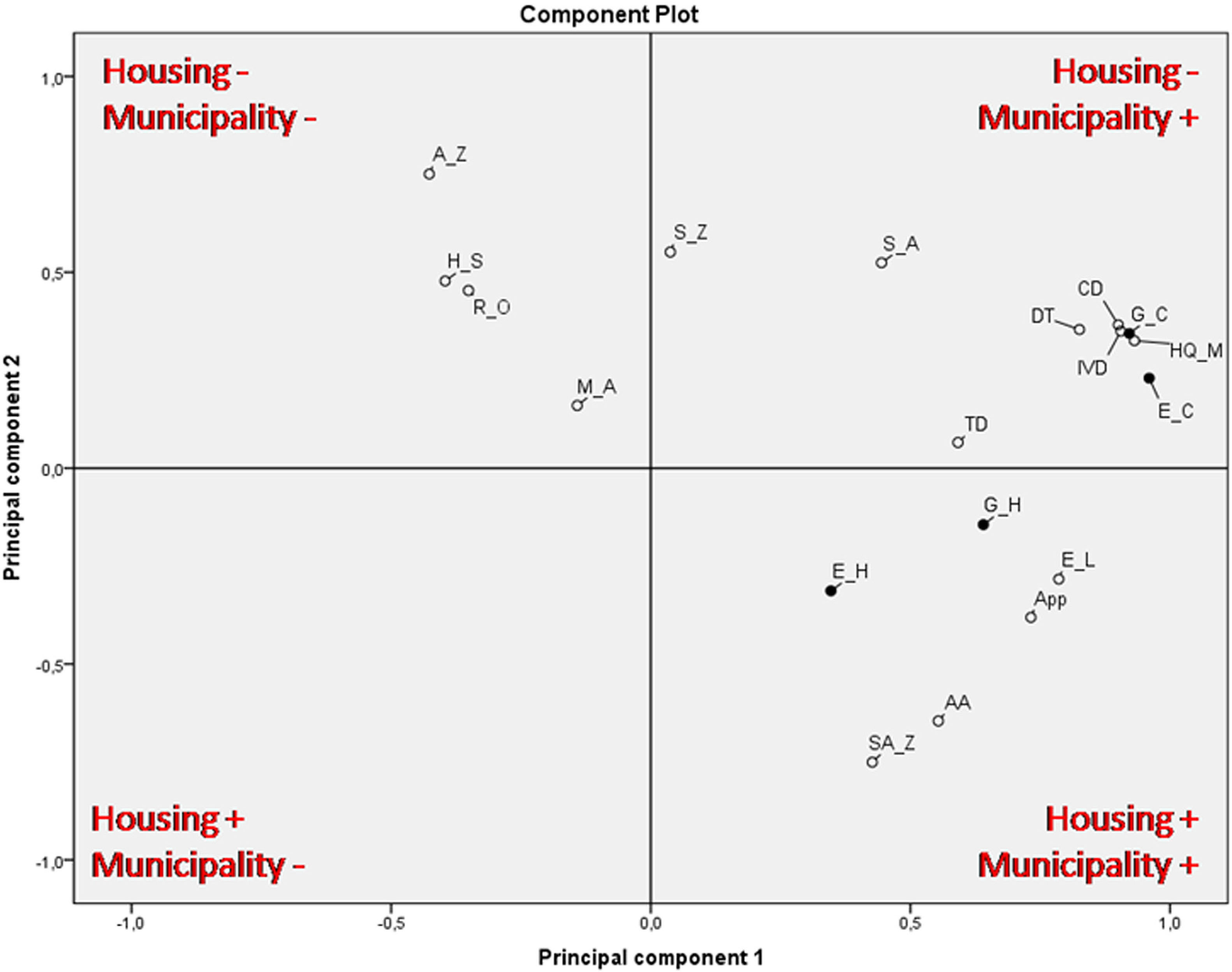
Fig. 6
PCA of all the variables used to cluster municipalities according to their population characteristics, dwelling typology, population distribution, climate zone, and appliance ownership.
Legend: A_Z = arid zone, SA_Z= semi-arid zone H_S = household size, R_O = room occupancy, M_A = mean area, HQ_M = population number living in headquarter municipality, S_Z = population number living in scattered zone, S_A = population living in secondary agglomeration, DT = density, CD = collective dwelling, IVD = individual dwelling, TD = traditional dwelling, G_C = gas consumption per municipality, E_C = electricity consumption per municipality, G_H = gas consumption per housing, E_H = electricity consumption per housing, E_L = education level, App = appliance ownership, AA = average age per housing per municipality.
Table 4
Characteristics of clusters.
| Cluster | 1 | 2 | 3 | 4 | ||
|---|---|---|---|---|---|---|
| Label | ▪ | ▾ | • | ♦ | ||
| Housing energy consumption | + | + | − | − | ||
| Municipality energy consumption | + | − | + | − | ||
| Size | 3 (8.3 %) | 26 (72.2%) | 1 (2.8 %) | 6 (16.7 %) | ||
| Variables | climate zone | semi-arid | semi-arid | semi-arid | arid | |
| population distribution | density | average density | low density | dense | low density | |
| municipality centre | moderately populated | thinly populated | highly populated | thinly populated | ||
| secondary agglomeration | moderately populated | thinly populated | thinly populated | thinly populated | ||
| scattered zone | moderately populated | moderately populated | moderately populated | highly populated | ||
| population characteristics | average age | highest rate | moderate rate | lowest rate | lowest rate | |
| education level | highest rate | low rate | moderate rate | low rate | ||
| dwelling occupancy | mean area | moderate | high | moderate | less | |
| room occupancy | moderate | moderate | highest rate | lowest rate | ||
| household size | low rate | moderate rate | lowest rate | highest rate | ||
| dwelling typology | collective dwelling | high rate | low rate | highest rate | lowest rate | |
| individual dwelling | high rate | low rate | highest rate | low rate | ||
| traditional dwelling | high rate | moderate rate | high rate | moderate | ||
| appliance ownership | highest rate | moderate rate | moderate rate | lowest rate | ||
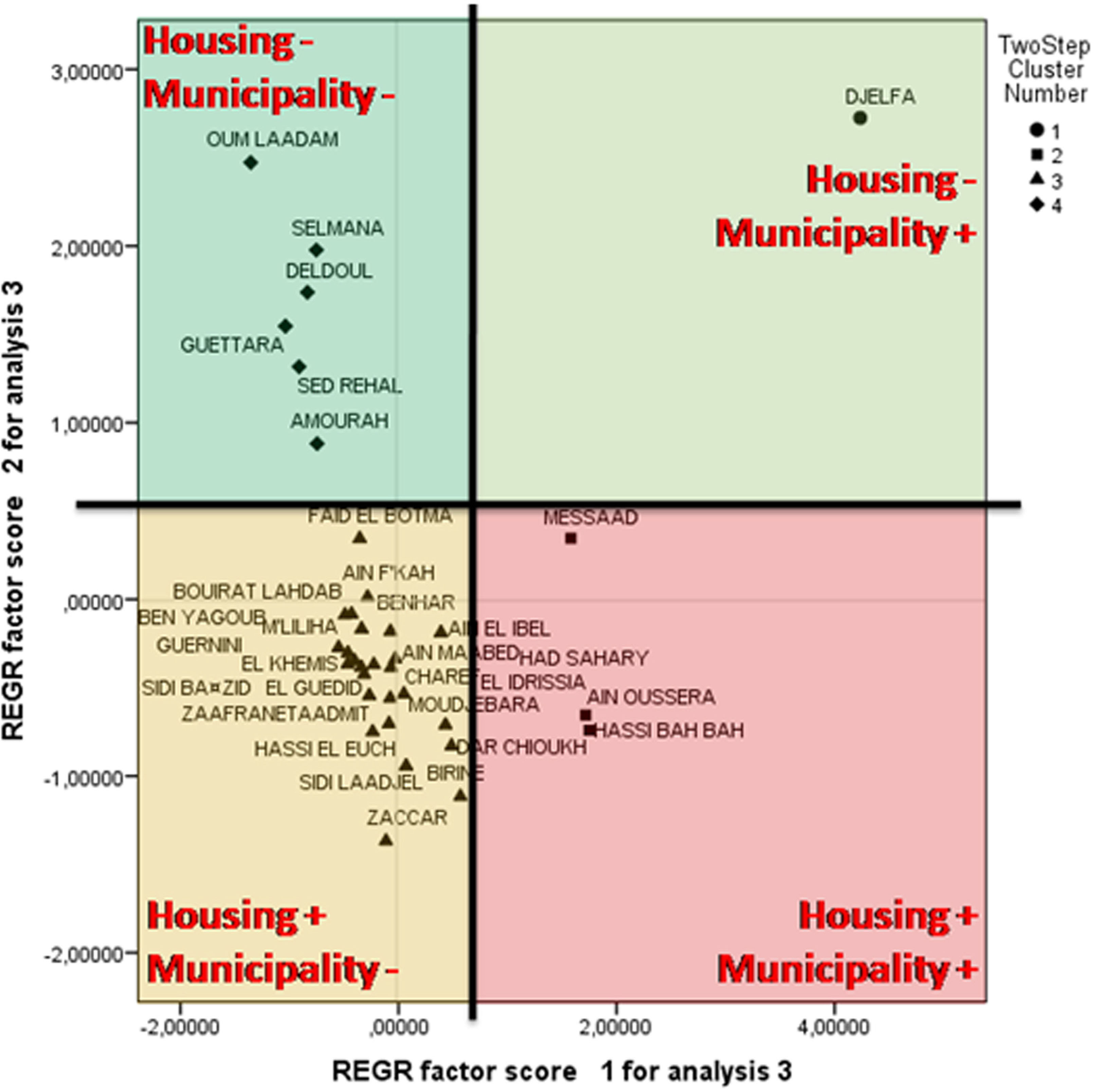
Fig. 7
Projection of municipalities according to PCA.
Table 5
Bivariate correlations between energy consumption and households, housing variables, density and appliance ownership.
| A-A | EL | Log10HRP>60 | M_A | H-S | R-O | Log10Dt | Log10 (A-C) | C | TV | Refr | WM | App | ||
|---|---|---|---|---|---|---|---|---|---|---|---|---|---|---|
| EUI | Correlation | .594** | .521** | .514** | −.593** | −.781** | −.321 | .335* | .280 | .348* | .490** | .358* | .253 | .431** |
| Sig. | .000 | .001 | .001 | .000 | .000 | .057 | .046 | .099 | .038 | .002 | .032 | .137 | .009 | |
| G | Correlation | .590** | .551** | .564** | −.543** | −.747** | −.330* | .395* | .287 | .390* | − | − | − | − |
| Sig. | .000 | .000 | .000 | .001 | .000 | .049 | .017 | .089 | .019 | − | − | − | − | |
| E | Correlation | .362* | .018 | −.166 | −.782** | −.746** | −.089 | −.356* | .086 | − | .078 | .044 | −.234 | .006 |
| Sig. | .030 | .916 | .332 | .000 | .000 | .604 | .033 | .616 | − | .653 | .800 | .170 | .973 | |
With, EUI: energy use index per capita (kwh/m2.y), G: household gas consumption per capita (kwh/m2.y), E: household electricity consumption per capita (kwh/m2.y), AA: average age, El: education level, Log10HRP>60 : log10 household with responsible person older than 60, M_A: mean area (m2), HS: household size, RO: room occupancy, Log10Dt: log10 density, Log10(A–C): log10 air conditioner, C: cooker ownership, TV: TV ownership, Refr.: refrigerator ownership, WM: washing machine ownership, App: mean appliance ownership.
Table 6
Model fit Indices of per-capita gas consumption.
| df | χ2 | Probability level | RMSEA | NFI | CFI | |
|---|---|---|---|---|---|---|
| gas model | 8 | 8.908 | 0.35 | 0.057 | 0.964 | 0.996 |
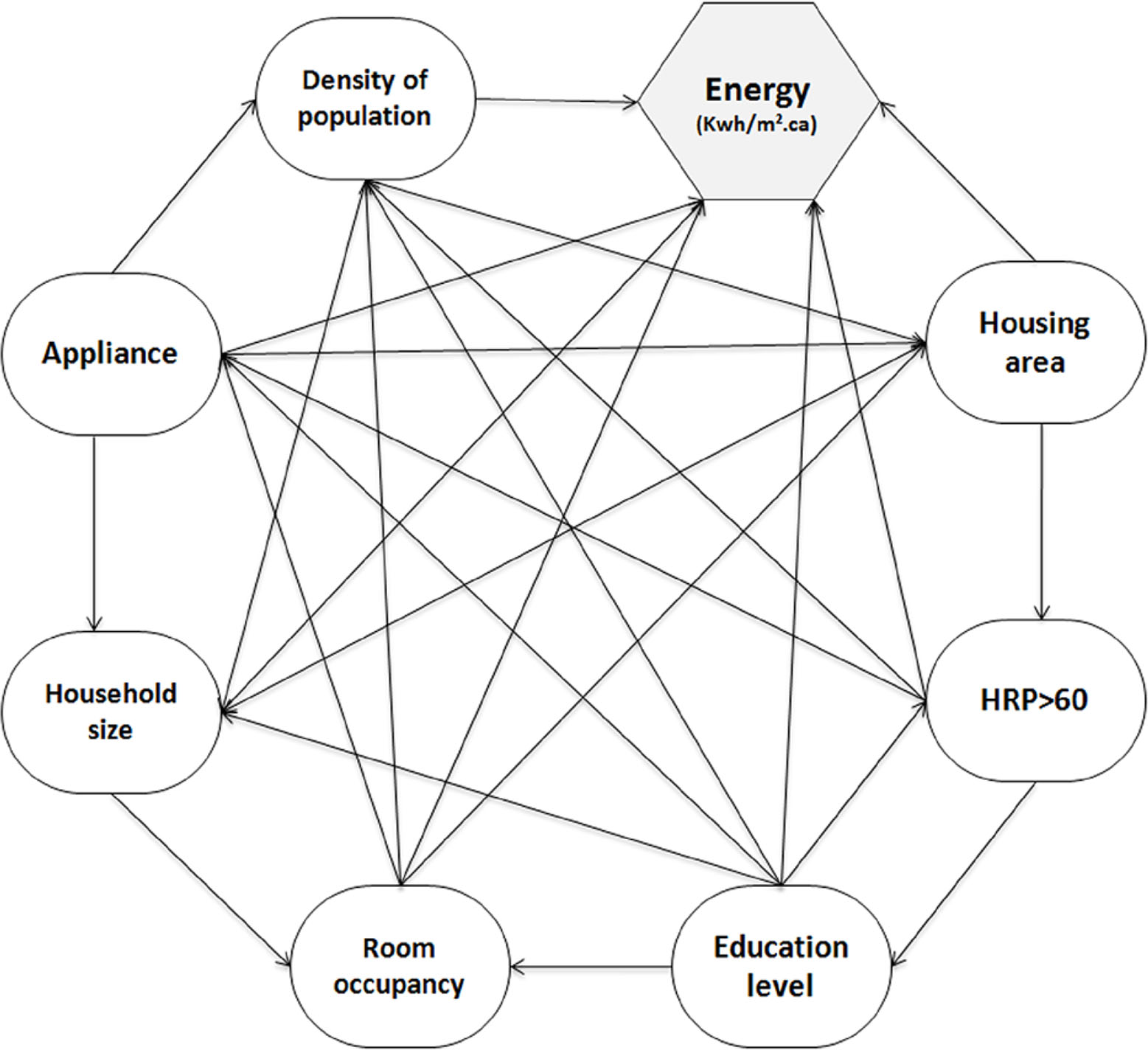
Fig. 8
Path analysis containing all possible hypotheses.
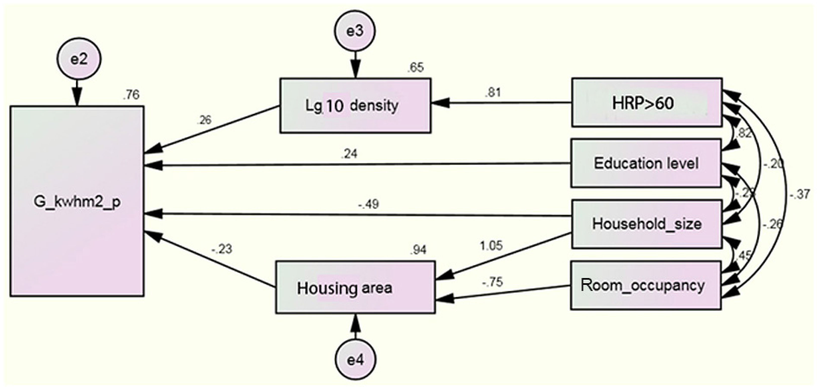
Fig. 9
Standardised direct effect for gas consumption per kwh/person.m2.y.
Table 7
Path analysis: standardised direct effect.
Table 8
Direct, indirect and total effect of household, housing and density variables on per-capita gas consumption.
| HRP>60 | Room Occupancy | Households size | Education Level | Housing area | Log 10 Density | |||||||||||||
|---|---|---|---|---|---|---|---|---|---|---|---|---|---|---|---|---|---|---|
| effect | Dir | Ind | tot | Dir | Ind | tot | Dir | Ind | tot | Dir | Ind | tot | Dir | Ind | tot | Dir | Ind | tot |
| M_A | .000 | .000 | .000 | −.745 | .000 | −.745 | 1.047 | .000 | 1.047 | .000 | .000 | .000 | .000 | .000 | .000 | .000 | .000 | .000 |
| density | .805 | .000 | .805 | .000 | .000 | .000 | .000 | .000 | .000 | .000 | .000 | .000 | .000 | .000 | .000 | .000 | .000 | .000 |
| gas* | .000 | .207 | .207 | .000 | .174 | .174 | −.493 | −.245 | −.738 | .239 | .000 | .239 | −.234 | .000 | −.234 | .257 | .000 | .257 |
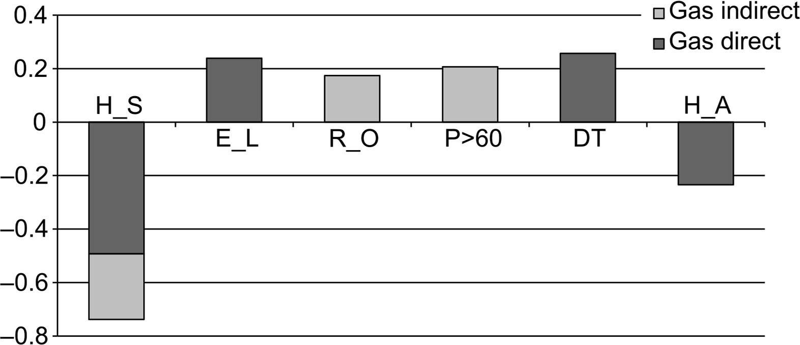
Fig. 10
Direct and indirect effect of variables on household gas consumption. With: H_S: household size, E_L: education level, R_O: room occupancy, HRP>60: household with a responsible person over the age of 60, DT: density, H_A: housing area.
Table 9
Electricity Model fit Indices.
| df | χ2 | Probability level | RMSEA | NFI | CFI | |
|---|---|---|---|---|---|---|
| Electricity model | 11 | 6.352 | 0.849 | 0.057 | 0.980 | 1.000 |
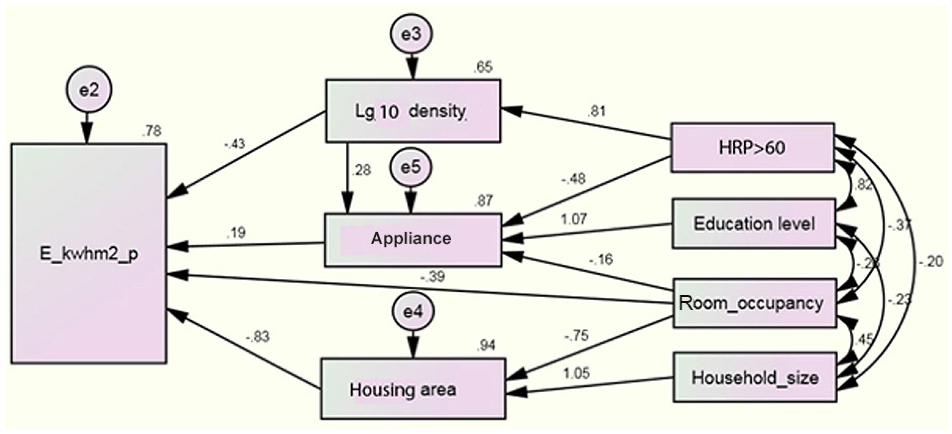
Fig. 11
Direct impact of variables on per-capita electricity consumption.
Table 10
Path analysis: significance of direct impact.
| Estimate | P | |||
|---|---|---|---|---|
| log 10 density | ← | HRP>60 | .805 | *** |
| appliance | ← | log density | .275 | .008** |
| appliance | ← | room occupancy | −.163 | .014** |
| appliance | ← | education local | 1.070 | *** |
| appliance | ← | HRP>60 | −.480 | *** |
| housing area | ← | room occupancy | −.745 | *** |
| housing area | ← | household size | 1.047 | *** |
| E_kwhm2_p | ← | housing area | −.829 | *** |
| E_kwhm2_p | ← | log density | −.430 | *** |
| E_kwhm2_p | ← | appliance | .194 | .071* |
| E_kwhm2_p | ← | room occupancy | −.395 | *** |
Table 11
Direct, indirect and total impact of variables on per-capita electricity consumption. Effect Household size Education level Room occupancy HRP>60 Log 10 density Appliance Housing area
| Effect | Household size | Education level | Room occupancy | HRP>60 | Log 10 density | Appliance | Housing area | ||||||||||||||
|---|---|---|---|---|---|---|---|---|---|---|---|---|---|---|---|---|---|---|---|---|---|
| Dir | indir | tot | Dir | indir | tot | Dir | indir | tot | Dir | indir | tot | Dir | indir | tot | Dir | indir | tot | Dir | indir | tot | |
| density | .000 | .000 | .000 | .000 | .000 | .000 | .000 | .000 | .000 | .805 | .000 | .805 | .000 | .000 | .000 | .000 | .000 | .000 | .000 | .000 | .000 |
| App | .000 | .000 | .000 | 1.070 | .000 | 1.070 | −.163 | .000 | −.163 | −.480 | .222 | −.259 | .275 | .000 | .275 | .000 | .000 | .000 | .000 | .000 | .000 |
| M_A | 1.047 | .000 | 1.047 | .000 | .000 | .000 | −.745 | .000 | −.745 | .000 | .000 | .000 | .000 | .000 | .000 | .000 | .000 | .000 | .000 | .000 | .000 |
| Elec* | .000 | −.868 | −.868 | .000 | .207 | .207 | −.395 | .586 | .192 | .000 | −.396 | −.396 | −.430 | .053 | −.376 | .194 | .000 | .194 | −.829 | .000 | −.829 |
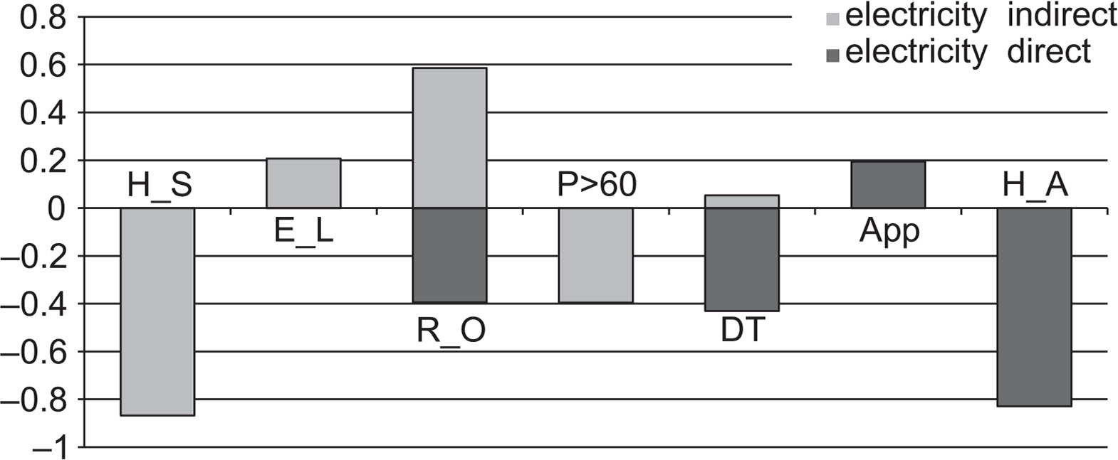
Fig. 12
Direct and indirect effect of variables on household electricity consumption. With: H_S: household size, E_L: education level, R_O: room occupancy, HRP>60: household with a responsible person over the age of 60, DT: density, App: appliance ownership, H_A: housing area.
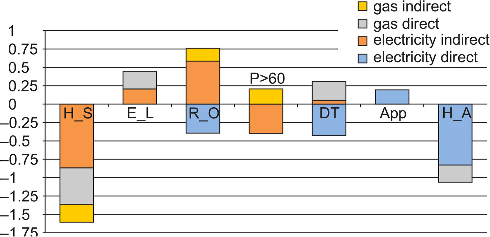
Fig. 13
Direct and indirect effect of variables on gas and electricity household consumption. With: H_S: household size, E_L: education level, R_O: room occupancy, HRP>60: household with a responsible person over the age of 60, DT: density, App: appliance ownership, H_A: housing area.