
Table 1.
Estimate of the number of qubits required to calculate R(5, 5) with Grover-style algorithm.
| n | Total qubits Q(n) (safe upper bound) | |
|---|---|---|
| 44 | 44 · 43/2 = 946 | 946 + 16 ≈ 962 |
| 45 | 45 · 44/2 = 990 | 990 + 16 ≈ 1006 |
| 46 | 46 · 45/2 = 1035 | 1035 + 16 ≈ 1051 |
| Coin-flip model | ↔ | Projector model |
|---|---|---|
| Indicator 1[mono-Kk] | ↔ | residual rank direction in M0 |
| First moment 𝔼X | ↔ | 𝔼 T(α), 𝔼 Tr Plin |
| Independence of edge colors | ↔ | i.i.d. isotropic vj |
| Counting patterns | ↔ | k rank–1 probes k in d dimensions |
| 𝔼X ≤ 1 threshold | ↔ | T(α) ↓ 0 and Pmiss ≪ 1 |
Table 2.
Trace of exponential projector, real and imaginary TrPexp, linear projector TrPlin, Minimum real eigenvalue of linear projector, Lyapunov exponent λL for each n at α = 20, k = 100, for n = 45 reports the best values obtained with α = 40 and k = 400. and slope of log10(Trace) vs. {α}. The symbol* = indicates a known limit solution for n = 5 used as test.
| n | 43 * | 44 | 45 | 46 |
|---|---|---|---|---|
| TrPexp | 7.92 × 10⁻¹² | 1.54 × 10⁻¹² | 10−289 ≈ 0 | 1.86 × 10⁻¹³ |
| TrPlin | 0.284 | 0.360 | 0.462 | 0.407 |
| min Reλ | –0.058 | –0.053 | –0.050 | –0.061 |
| max Imλ | ±0.037 | ±0.030 | ±0.032 | ±0.063 |
| λL | 1.55 | 1.48 | 1.41 | 1.54 |
| Slope | –0.674 | –0.642 | –0.612 | –0.670 |
Table 3.
Prime–sparse extrapolation of the unknown diagonal values R(6, 6) and R(7, 7).
| Ramsey N. | 𝒫5 | 𝒫6 | 𝒫7 | 𝒫8 | 𝒫9 | 𝒫10 | 𝒫11 | 𝒫12 | 𝒫13 |
|---|---|---|---|---|---|---|---|---|---|
| R(6, 6) | 108 | 108 | 117 | 117 | 115 | 115 | 115 | 111 | 111 |
| R(7, 7) | 225 | 216 | 221 | 209 | 209 | 209 | 209 | 209 | 205 |
Table 4.
R(5, 5) under k ≤ 2n – 1 (n = 5): admissible and selected values as 𝒫k grows.
| R(5, 5) k | prime set | admissible integers in (43, 46] |
|---|---|---|
| 3–5 | 𝒫3–5 (11 and 23 absent) | 45 = 325 |
| 5–8 | 𝒫5–8 (11 present) | 44 = 2211, 45 = 325 |
| 9 | (23 present) | 44, 45, 46 = 2·23 |
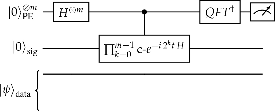
Figure 1.
Phase-estimation on the Hermitian dilation H (Eq. (23)) to estimate its extremal eigenphase(s), hence . The “sig” (sign) qubit together with the data register realizes the 2d-dimensional space of the dilation; the PE register controls powers of e−itH. A local maximum of the extracted at the critical v complements the linear/exponential diagnostics.
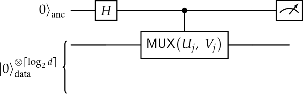
Figure 2.
One-ancilla rank-1 block-encoding gadget Wj implementing the top-left block (see Eq. (24)). The multiplexor applies Uj when the ancilla is |0〉 and Vj when it is |1〉. Composing these gadgets with a single selector/index register and oblivious amplitude amplification yields an α0–block-encoding of .
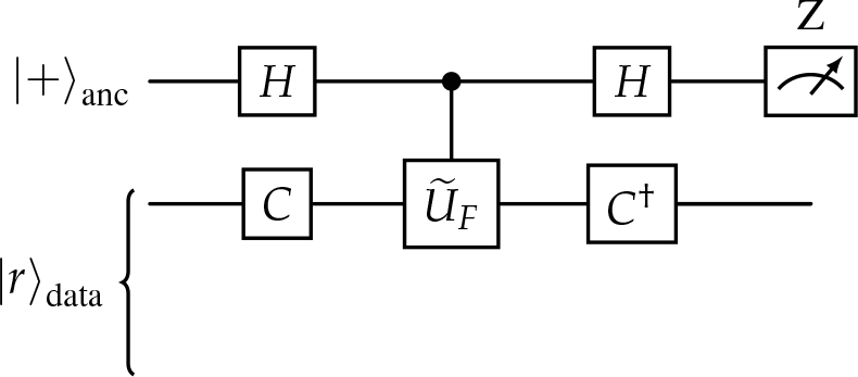
Figure 3.
Hadamard-test realization of the Hutchinson identity (Eq. (25)). A random |r〉 is prepared by a unitary 2-design C on the data register; is a block-encoding of F (either F = Pexp (α) = e−aA or F = Plin). Averaging the ancilla’s 〈Z〉 over random |r〉 gives an unbiased estimate ofTr F/d; amplitude estimation can reduce shot complexity.
Table A1.
Upper bounds on Pmiss from Eq. (A16) for the parameters used in our numerical study.
| Surviving rank r | Mean hits kp = rk/d | Bound on Pmiss | log10 Pmiss |
|---|---|---|---|
| 1 | 4.17 | 1.2 × 10⁻¹ | –0.9 |
| 2 | 8.33 | 4.0 × 10⁻² | –1.4 |
| 4 | 16.67 | 3.7 × 10⁻³ | –2.4 |
| 6 | 25.00 | 3.4 × 10⁻⁴ | –3.5 |
| 8 | 33.33 | 3.0 × 10⁻⁵ | –4.5 |
| 10 | 41.67 | 2.7 × 10⁻⁶ | –5.6 |
| 12 | 50.00 | 2.5 × 10⁻⁷ | –6.6 |
Table A2.
Diagnostic values for the explicit 46-vertex coloring. For comparison, the rightmost column reproduces the ensemble averages (the Angeltveit–McKay, AM–46, coloring [3]) reported earlier for generic n = 46 instances.
| explicit AM-46 | bulk average (n = 46) Tab I | |
|---|---|---|
| Tr Plin | 0.409 ± 0.004 | 0.407 |
| min Reλ Plin) | –0.060 | –0.061 |
| max |Imλ| | 0.032 | 0.063 |
| ReTrPexp | +1.79 × 10⁻¹³ | +1.86 × 10⁻¹³ |