
Table 1.
State transition table for a simple non-deterministic machine.
| Present State (PS) | Next State (NS) |
|---|---|
| S0 | S1 |
| S1 | S2 |
| S2 | S0 |
| S3 | S0, S1, S2 |
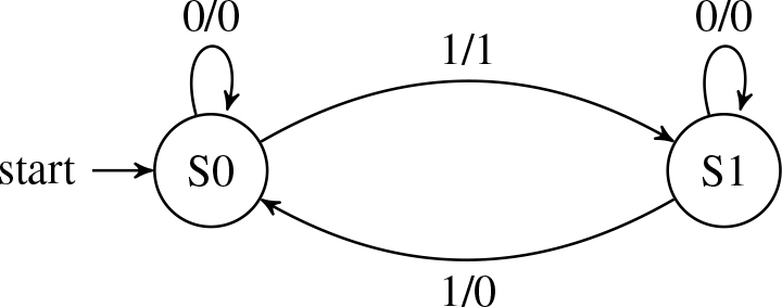
Figure 1.
DFA which provides the input-output response shown in Table 2.
Table 2.
Example Input-Output Traces.
| Trace # | Input | Output |
|---|---|---|
| 1 | 000000 | 000000 |
| 2 | 000001 | 000001 |
| 3 | 000101 | 000100 |
| 4 | 010011 | 010001 |
| 5 | 100010 | 100000 |
| 6 | 111000 | 101000 |
| 7 | 110101 | 100100 |
| 8 | 111110 | 101010 |
Table 3.
Input-Output Trace for a machine that detects a 1 in the third from last symbol of a string.
| Trace # | Input | Output |
|---|---|---|
| 1 | 0000 | 0000 |
| 2 | 1000 | 0001 |
| 3 | 000101 | 000000 |
| 4 | 011011 | 000001 |
| 5 | 011100 | 000001 |
| 6 | 1110001 | 0000000 |
| 7 | 1111001 | 0000001 |
| 8 | 111110111 | 000000000 |
| 9 | 000001000 | 000000001 |
| ‥ | ……… | ……… |
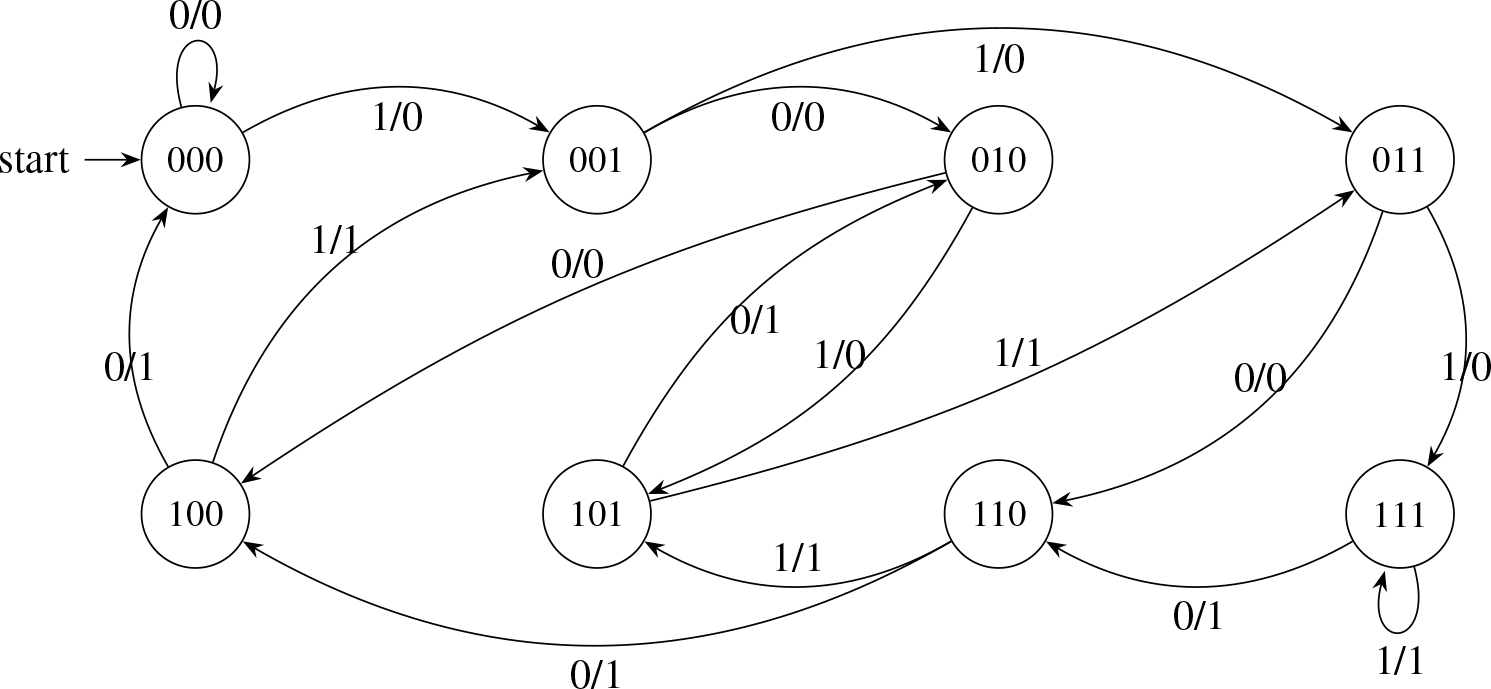
Figure 2.
DFA for detecting a 1 in the third from last position of an input string of length L. Each state encodes the last three input bits. On input x, the output is the oldest bit of the window (the 3rd-from-last).
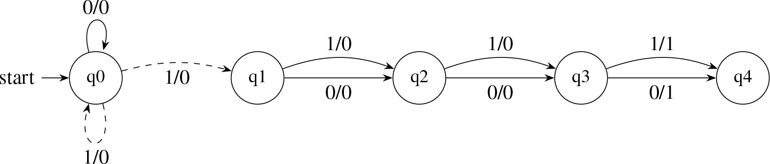
Figure 3.
NFA for detecting a 1 in the third from last position of an input string of length L. The dotted arcs indicate non-deterministic transitions.
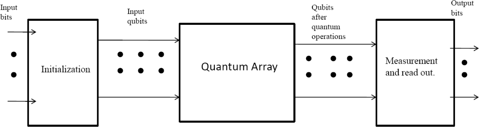
Figure 4.
Quantum State Machines with State Retention (QSM-SR). Inputs are classical bits that are used to initialize some qubits. Quantum operations are performed on these qubits by the array. After each pass through the array, the states are retained by the qubits. Thus the state qubits do not get re-initialized after the first pass through the array, while some inputs may get re-initialized before every pass through the array.
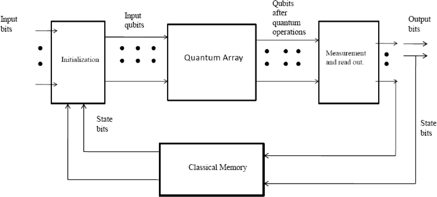
Figure 5.
Quantum State Machines with Classical Memory (QSM-CM). Inputs are classical bits that are used to initialize some qubits. Quantum operations are performed on these qubits by the array. After each pass through the array, the states are read out and stored in a classical memory. These state bits are used to re-initialize some qubits before the next pass through the array.
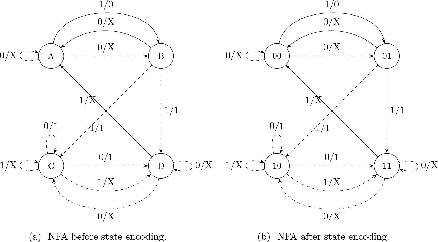
Figure 6.
Non-deterministic finite automaton with some outputs as don’t cares.
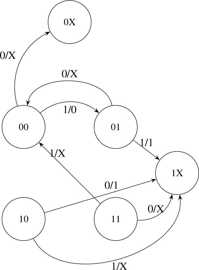
Figure 7.
Non-deterministic finite automaton with some outputs and states as don’t cares.
Table 4.
State transition table that represents the operation of the non-deterministic automaton in Figure 7 as an incompletely specified 3 × 3 function.
| Present State Inputs Q1Q2In (ABC) | Next State Outputs Q′1Q′2Out (PQR) |
|---|---|
| 000 | 0XX |
| 001 | 010 |
| 010 | 00X |
| 011 | 1X1 |
| 100 | 1X1 |
| 101 | 1XX |
| 110 | 1XX |
| 111 | 00X |
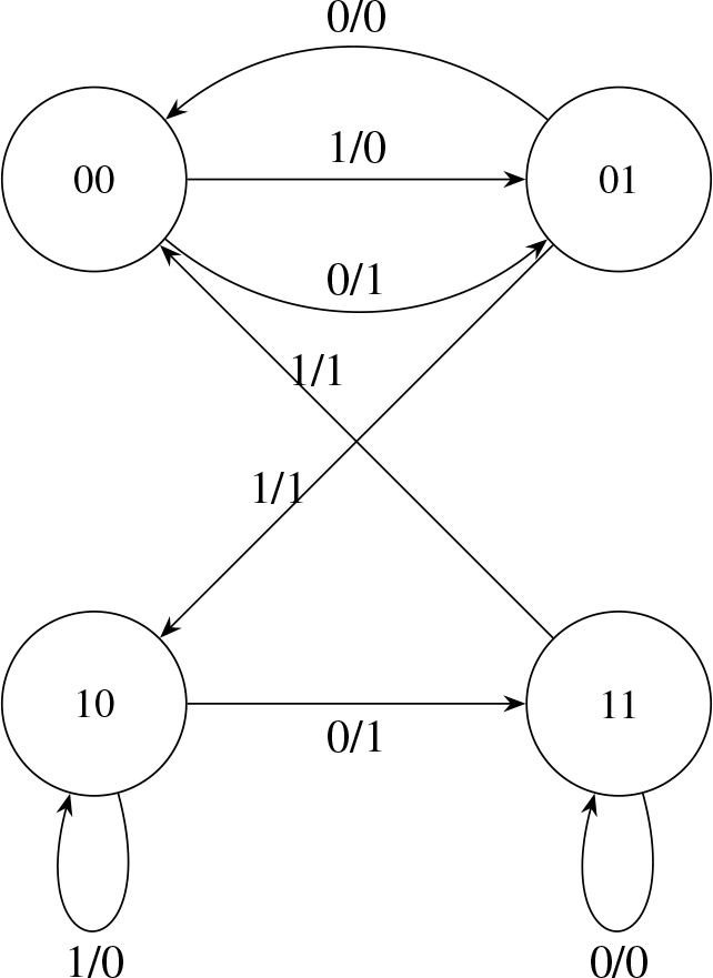
Figure 8.
Deterministic automaton with state transition table that is consistent with the non-deterministic automaton in Figure 6.
Table 5.
State Transition Table that represents the operation of the automaton in Figure 8 as a completely specified 3 × 3 function.
| Present State Inputs Q1Q2In (ABC) | Next State Outputs Out Q′1Q′2Out (PQR) |
|---|---|
| 000 | 011 |
| 001 | 010 |
| 010 | 000 |
| 011 | 101 |
| 100 | 111 |
| 101 | 100 |
| 110 | 110 |
| 111 | 001 |
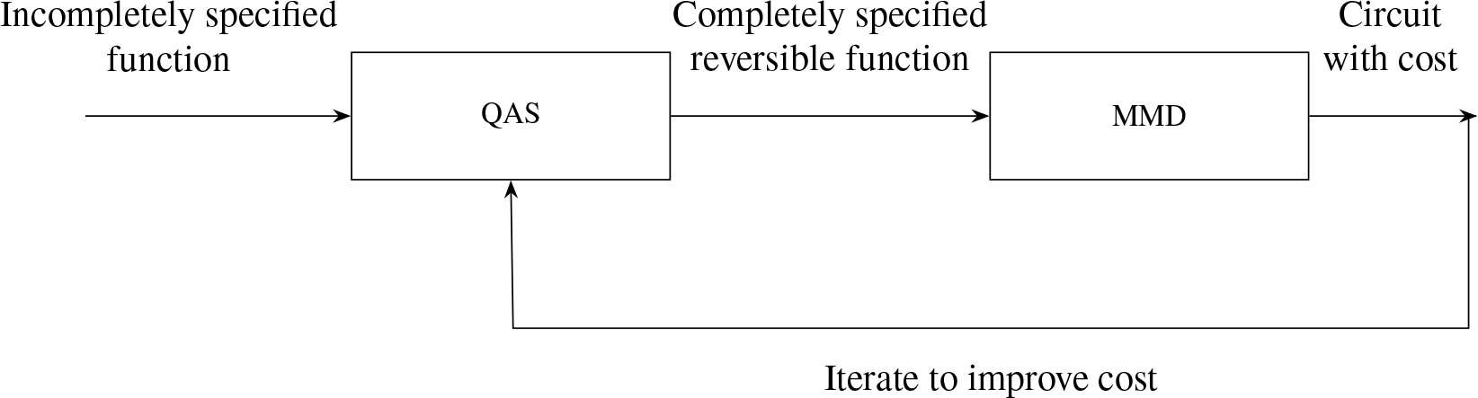
Figure 9.
Black box model of the QAS system. The input and output of QAS are in the form of truth tables, incompletely specified and completely specified, respectively.
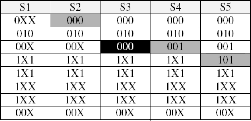
Figure 10.
QAS outputs, steps S1–S5.
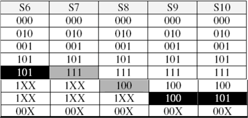
Figure 11.
QAS outputs, steps S6–S10.
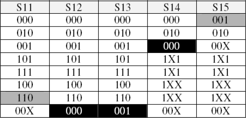
Figure 12.
QAS outputs, steps S11-S15.
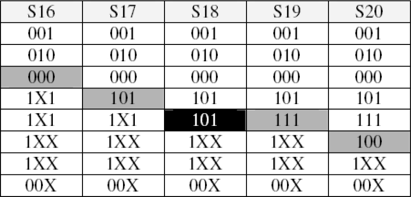
Figure 13.
QAS outputs, steps S16-S20.
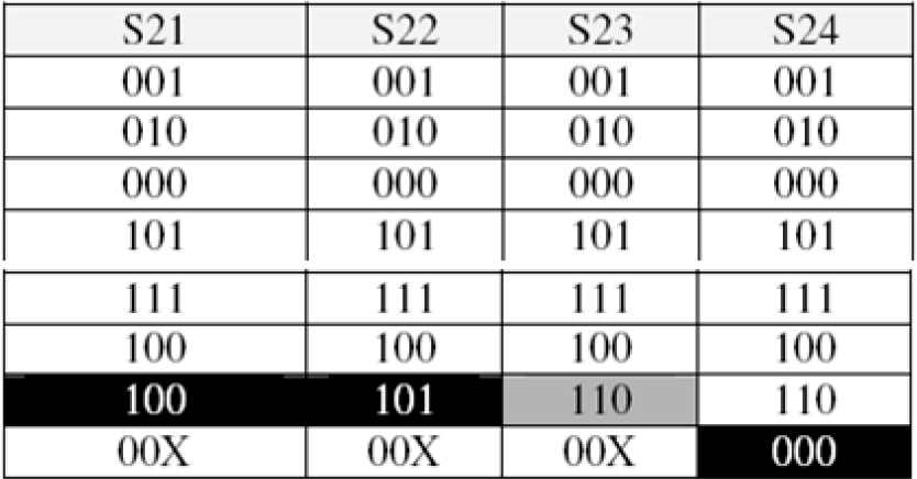
Figure 14.
QAS outputs, steps S21-S24.
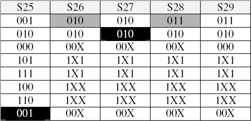
Figure 15.
QAS outputs, steps S25-S29.
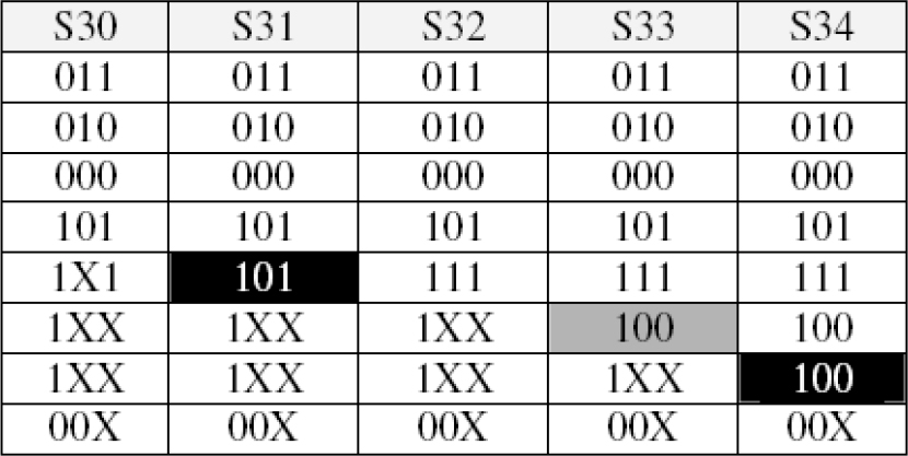
Figure 16.
QAS outputs, steps S30-S34.
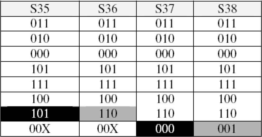
Figure 17.
QAS outputs, steps S35-S38.
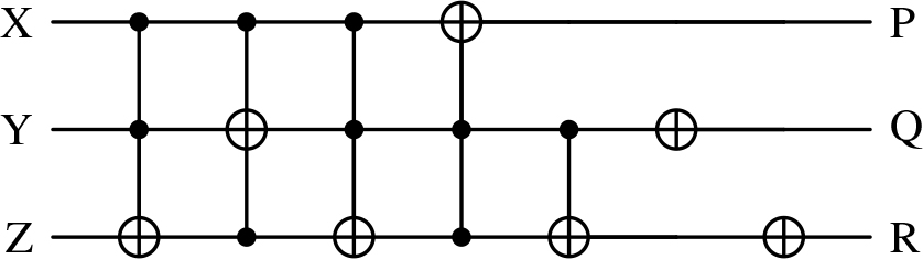
Figure 18.
Final Circuit for realization of transition and output functions for automaton from Figure 6, assuming no ancilla qubits.
Table 6.
Original function versus final function f(A,B,C) after QAS application.
| Inputs (ABC) | Original Outputs (PQR) | Final Outputs (PQR) |
|---|---|---|
| 000 | 0XX | 011 |
| 001 | 010 | 010 |
| 010 | 00X | 000 |
| 011 | 1X1 | 101 |
| 100 | 1X1 | 111 |
| 101 | 1XX | 100 |
| 110 | 1XX | 110 |
| 111 | 00X | 001 |
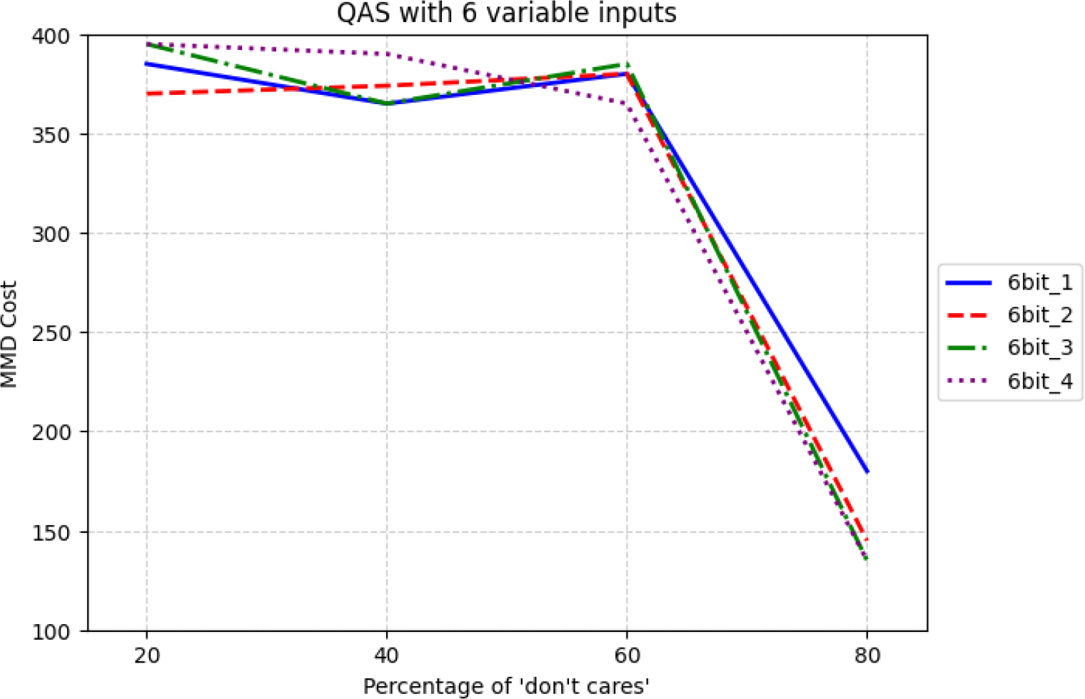
Figure 19.
QAS trend of MMD cost versus percentage of don’t cares for four 6-qubit benchmark functions.
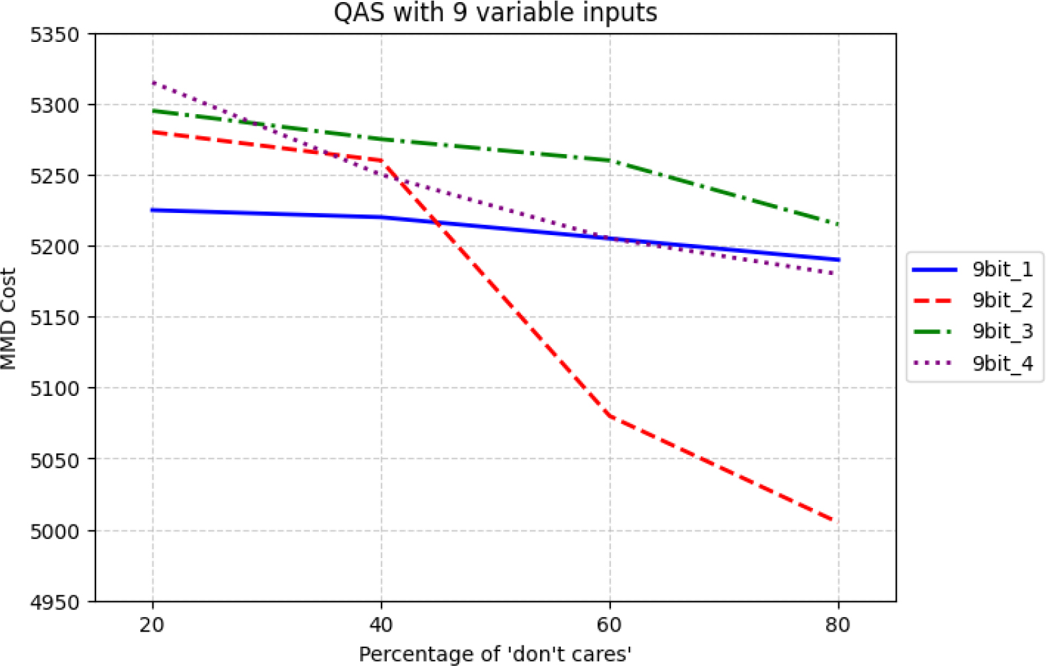
Figure 20.
QAS trend of MMD cost versus percentage of don’t cares for four 9-qubit benchmark functions.
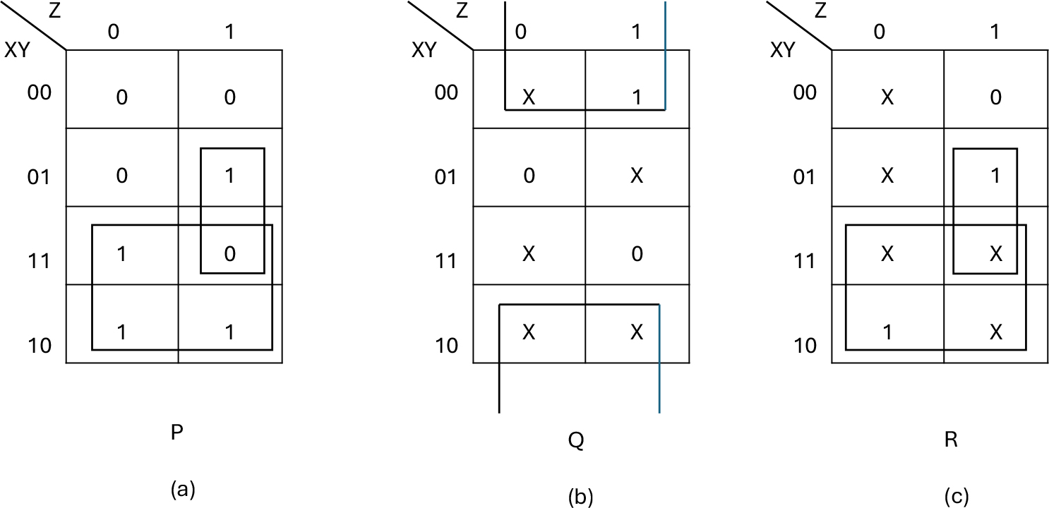
Figure 21.
Karnaugh maps that represent the transition and output functions for the state machine in Table 4. (a) P = X ⊕ YZ (b) Q = Y ′ and (c) R = X ⊕ YZ
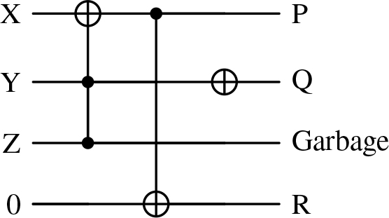
Figure 22.
Circuit to realize transition and output functions for automaton from Figure 6 assuming one ancilla qubit.