
The development of large-scale quantum computers will have a significant impact on the security of many cryptographic schemes currently in use [1]. In particular, the introduction of Shor’s algorithm [2,3] can solve factorization and discrete logarithm problems in polynomial time. Since almost all current public key schemes are built on the assumption of these computationally difficult problems, this will have a devastating impact on asymmetric cryptographic schemes. This situation has triggered a new line of research, namely post-quantum cryptography, which aims to develop new cryptographic primitives in the hope of resisting attackers equipped with quantum computers. NIST has proposed the post-quantum asymmetric scheme project [4–7] to standardize several quantum-resistant publickey cryptographic algorithms. It is crucial to start the transition to quantum-resistant cryptography before quantum computers are truly available. Fully exploring the potential of quantum algorithms to attack cryptographic schemes and effectively assessing the quantum security of existing schemes under quantum computing will help better design cryptographic algorithms to resist attacks from future quantum computers.
However, the situation for symmetric cryptographic schemes is less clear: universal attacks define the security of ideal symmetric primitives and will achieve a quadratic speed-up through Grover’s algorithm [8,9], implying that in a post-quantum world, doubling the key length can restore equivalent ideal security. For nearly 20 years, it was believed that Grover’s algorithm was the only advantage attackers had when attacking symmetric cryptography using quantum computers. Although the community seems to think that this solution [10,11] has solved the problem, knowledge about practical attacks is still very limited. At present, the impact of many quantum attacks on symmetric cryptography remains unclear, and potential threats need to be explored. The National Academy of Sciences report on the rise of quantum computing [12] also pointed out that there may be some currently unknown clever quantum attacks, such as Simon’s algorithm. Indeed, cryptographers have made significant progress against quantum attackers using superposition queries, which can break many symmetric key schemes in polynomial time.
Quantum algorithms have become a central focus in the field of symmetric cryptanalysis. Grover’s algorithm is one of the most widely applied algorithms in this field, as it can speed up the search efficiency in an unstructured database of size 2n, reducing the complexity of exhaustive search attacks from 𝒪(2n) to
In recent years, a significant focus of research has been the development of new quantum attack algorithms targeting cryptographic schemes. One popular approach involves combining different quantum algorithms to achieve more efficient attacks, such as Grover-meets-Kuperberg algorithm [28], Bernstein–Vazirani-meets-Grover algorithm [29], etc. The Grover-meets-Simon algorithm proposed by Leander and May [30] is the most widely applied among them, where Grover’s algorithm serves as the outer structure and Simon’s algorithm as the inner structure. The period identified by Simon’s algorithm is used as the decision condition of Grover’s search. The introduction of the Grover-meets-Simon has enabled its application to search for two keys in function structures that can be modeled as periodic functions [31–33]. Building on this idea, Bonnetain [34] proposed two improved combinations of Grover’s algorithm and Simon’s algorithm under the Q1 model (attackers perform offline quantum computations but make only classical online queries) and Q2 model (attackers can make superposition queries to a quantum oracle), where the one in the Q2 model is called Alg-PolyQ2 algorithm. This Alg-PolyQ2 algorithm leverages a combination of online queries and offline computation to achieve an exponential reduction in quantum query complexity.
Despite the promising structure of these combined quantum algorithms, the actual attack success probability and the required number of iterations, especially under practical constraints such as deferred measurement, remain insufficiently characterized. This motivates our work: to analyze in detail how the internal structure of these algorithms affects their success probability under deferred measurement, and to derive tight bounds on the attack success probability and the required number of iterations. Through this analysis, we aim to better understand the real-world effectiveness of such combined quantum attacks, going beyond asymptotic query complexity and providing quantitative insight into their feasibility.
Our contributions In this paper, we mainly study the Grover-meets-Simon and Alg-PolyQ2 algorithms in detail under deferred measurement. We analyze the generalized success probability of these two algorithms in detail from a novel perspective based on the initial amplitude, thereby confirming their effectiveness. To the best of our knowledge, such a detailed analysis has not been done before. In more detail, our main contributions are as follows:
Since both algorithms involve the rank-solving problem of a system of linear equations, we provide a formal analysis of the generalized quantum Gauss-Jordan elimination. Through the formal description, we discuss the situation (quantum state form) of obtaining the reduced row echelon form matrix based on this method, demonstrate the necessity of auxiliary qubits, and provide its formal proof. Based on the deferred measurement principle to solve the rank, we further analyze the rank-solving process and provide the number of matrices with rank-(n – 1) in both n-dimensional and (n – 1)-dimensional linear spaces, respectively, along with the corresponding proofs. This is the first time to consider in detail the formal analysis of quantum Gauss–Jordan elimination as a subroutine to solve the rank in the parallel Simon’s algorithms under deferred measurement.
We provide a tight analysis of the Grover-meets-Simon and Alg-PolyQ2 algorithms under deferred measurement in detail. Specifically, considering that when Simon’s algorithm is used as the internal structure, the key space will collapse if the intermediate measurements are made. Therefore, combined with the deferred measurement principle, we examine the challenges arising from deferring all measurements in Simon’s algorithm to the end of the entire computation during the iteration process. Based on the oscillation amplitude of the initial state, the tight bounds of the generalized success probability and the optimal number of iterations of the Grover-meets-Simon algorithm are analyzed in detail. Similarly, we also provide a tight analysis of the Alg-PolyQ2 algorithm to demonstrate its effectiveness as a quantum attack. This paper provides a novel perspective for assessing the practical effectiveness of quantum algorithms—one that does not rely on assumptions about quantum input length, such as the number of parallel instances of Simon’s algorithm and the choice of plaintext pairs in the classifier of the Grover-meets-Simon algorithm.
Outline The rest of the paper is organized as follows: Section 2 introduces the relevant knowledge of quantum circuit models and quantum algorithms; Section 3 provides a formal analysis of the generalized quantum Gauss-Jordan elimination; Section 4 provides a tight analysis of the Grover-meets-Simon and Alg-PolyQ2 algorithms under deferred measurement via formalizing quantum rank-solving; Section 5 discusses some future research directions; Section 6 summarizes this paper.
In this section, we introduce some concepts of quantum computation and review Simon’s and Grover’s algorithms.
A circuit consisting of a series of quantum gates applied to a group of qubits is called a quantum circuit, which can be used to describe the change of quantum state in Hilbert space. Each quantum logic gate can be represented by a unitary matrix. These unitary operators in Hilbert space are all invertible, and it may be necessary to use enough auxiliary qubits to achieve the required goal. A single qubit has two quantum ground states |0〉, |1〉. If the quantum state |φ〉 can be linearly represented by |0〉, |1〉, then this state is called a superposition state |φ〉 = α|0〉 + β|1〉. Among them, the probability amplitudes α and β are complex numbers, and |α|2 + |β|2 = 1. When an n-qubit is given, the computational basis has 2n vectors. After applying a series of quantum gates to the initial state, the original superposition state changes. Finally, the system is measured and some n-qubit vectors are obtained on the computational basis to get the desired result.
Quantum computing takes advantage of parallel computing by utilizing quantum phenomena such as quantum superposition and entanglement, allowing multiple computable states to be processed simultaneously, thereby improving efficiency and speed. The unique capabilities of quantum computers enable them to surpass classical computers in certain computing tasks.
Assume f(x) : {0,1}n → {0,1}m, the mapping of this function in the quantum setting can be used as an oracle Uf : |x, y〉 → |x, y ⊕ f(x)〉. When the initial state |0〉⊗n|0〉⊗m is input,
In addition, the following two important principles regarding quantum circuits are very practical. For detailed proof, refer to [35].
Measurements can always be moved from the intermediate stage of a quantum circuit to the end of the circuit. Any measurement that occurs inside a quantum circuit can be deferred to the end of the circuit.
Any unmeasured qubit at the end of a quantum circuit can be assumed to be measured.
Simon’s algorithm [19] aims to solve the periodic problem of hidden subgroups, which can be described as follows:
Simon’s Problem with promise: suppose there is a quantum oracle to a function f: {0,1}n → {0,1}m such that ∃ s ∈ {0,1}n, ∀ x ∈ {0,1}n, f(x) = f(x ⊕ s). The goal is to find the period s.
An individual Simon’s algorithm can be performed by the following steps, with the corresponding quantum circuit shown in Figure 1.
Prepare the initial state
|0\rangle _I^{ \otimes n}|0\rangle _{II}^{ \otimes m} {1 \over {\sqrt {{2^n}} }}\sum\limits_{x \in {{\{ 0,1\} }^n}} | \;x{\rangle _I}|0{\rangle _{II}}. Perform a quantum query on the function f, mapping to the following quantum state:
{1 \over {\sqrt {{2^n}} }}\sum\limits_{x \in {{\{ 0,1\} }^n}} | \;x{\rangle _I}|f(x){\rangle _{II}}. Perform the Hadamard transform H⊗n on the first register, and the following quantum state can be obtained:
{1 \over {{2^n}}}\sum\limits_{y \in {{\{ 0,1\} }^n}} {\sum\limits_{x \in {{\{ 0,1\} }^n}} {{{( - 1)}^{x\;\cdoty}}} } |y{\rangle _I}|f(x){\rangle _{II}}. Suppose there is some s ≠ 0, for each y, then |y, f(x)〉 = |y, f(x ⊕ s〉, and the amplitude of this configuration is:
1 \alpha (x,y) = {1 \over {{2^n}}}\left[ {{{( - 1)}^{x\;\cdoty}} + {{( - 1)}^{(x \oplus s)\cdoty}}} \right] = {1 \over {{2^n}}}{( - 1)^{x\;\cdoty}}\left[ {\left( {1 + {{( - 1)}^{s\;\cdoty}}} \right].} \right. Let X1 be an ((n – 1)-dimensional subspace of
_2^n _2^n s \in _2^n\backslash {X_1} Measure the first register, and it will collapse to a value that satisfies y · s = 0.
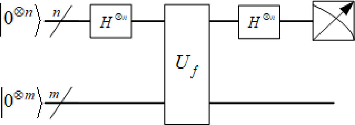
Quantum circuit of Simon’s algorithm.
When y · s = 1, the amplitude of α(x, y) is 0. Hence, we can only get the vector y orthogonal to period s. The parallel Simon’s algorithms under deferred measurement only need 𝒪(n) oracle queries, n – 1 linearly independent values of y are obtained with high probability, then s can be obtained by solving the following linear equations:
Simon’s algorithm is a probabilistic algorithm, and the promise of Simon’s problem is not always fully satisfied in cryptanalysis. We introduce a theorem to quantify the relationship between the number of parallel instances of Simon’s algorithm and the success probability. The proof can be found in [23]:
Given f : {0,1}n → {0,1}m and s as an actual period of f, ∃ t ∈ {0,1}n\{0, s} such that the input x ∈ {0,1}n satisfies f(x ⊕ t) = f(x). Define
If ε(f) ≤ p0 < 1, after performing l instances of Simon’s algorithm in parallel, the success probability of outputting the actual period s is at least
Grover’s algorithm [8,9] aims to quickly search for r marked solution elements in an unstructured database of size N, which can achieve a quadratic speedup compared to the time complexity of classical exhaustive algorithms. It can be described as follows:
Grover’s problem: given a search space N whose elements are represented on n = log2 N qubits, suppose there is a quantum oracle to a function f: {0,1}n → {0,1} such that x ∈ N, f(x) = 1. The goal is to find these r marked solution elements.
Amplitude amplification is a natural generalization of the original Grover’s algorithm. The result of amplitude amplification is described in the following theorem [13], with the corresponding quantum circuit shown in Figure 2.
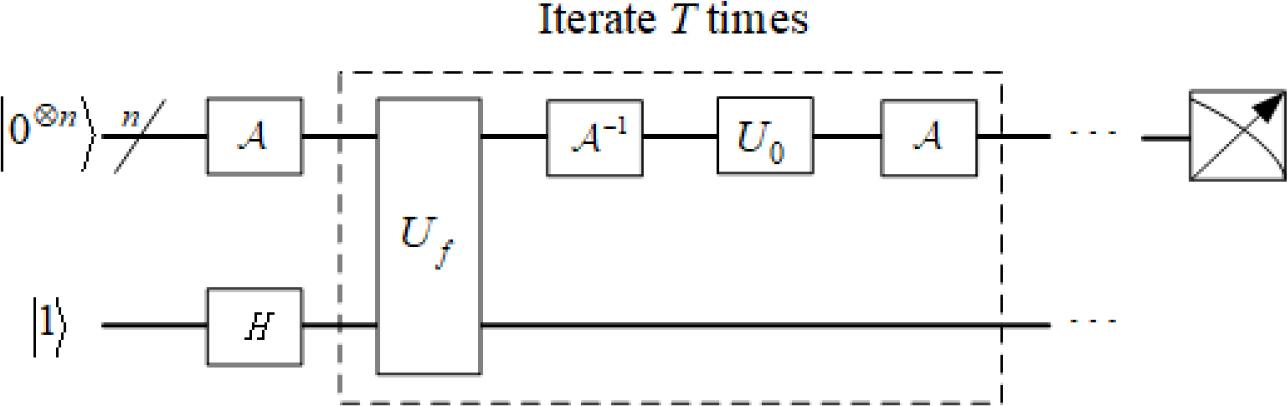
Quantum circuit of generalized Grover’s algorithm.
Here, 𝒜 is the Hadamard transform H⊗n in the original Grover’s algorithm.
Let 𝒜 be any quantum algorithm without measurement, and let f: {0, 1}n → {0, 1} be a Boolean function that distinguishes between good and bad states from the output of the algorithm 𝒜. Let p > 0 be the initial success probability of 𝒜|0〉. We define 𝒬 = –𝒜U0𝒜−1Uf, where U0 = 2|0〉⊗n〈0|⊗n – I, Uf is performed:
After T iterations 𝒬T 𝒜|0〉, the outcome is good with probability at least max {p, 1 – p} under deferred measurement, where
Quantum Gauss-Jordan elimination (QGJE) was first proposed by Do et al. [36] to solve the linear system of n equations on n variables AX = b, aij ∈ A, with the goal of achieving a speedup over classical computing techniques. However, no formal proof has been provided yet. In this section, we provide a formal analysis of the generalized QGJE, in particular the existence of a full rank or rank-(n – 1) check in a quantum oracle of cryptographic algorithms. The following are the formal steps to perform it. For detailed quantum gate operations of the generalized QGJE, please refer to [37,38].
Given a quantum coefficient matrix
Step 1: First, find out the first non-zero |ai,1〉 ≠ 0 using Grover’s Search algorithm.
Step 2: If successful, take the first leading |1〉 in the first position as |a1,1〉, otherwise change to the next column and repeat step 1.
Step 3: Eliminate all other elements |a2,1〉, ⋯, |an,1〉, in the first column.
Step 4: Change n to n – 1, control if still n > 0, repeat step 1.
Step 5 In backward eliminate all |an–1,n〉, ⋯, |a1,n〉.
Step 6: Check if n > 0, change n to n – 1, and repeat step 5.
The QGJE is chosen because it is a generalized quantum extension of the classical Gauss-Jordan elimination, which serves as the foundational algorithm for rank-solving problems. The algorithm proposed by Bonnetain and Jaques is specifically tailored to determine the full-rank property of certain structured matrices derived from symmetric cryptographic primitives and its core technique still relies on Gauss-Jordan elimination to transform the matrix into an upper triangular form. The quantum algorithms proposed by Xia et al. are universal and can compute both the rank and the general solution of arbitrary quantum linear systems with a single measurement. Therefore, for the detailed steps of quantum rank-solving, please refer to [37,38].
In brief, if the rank is required through deferred measurement, then these auxiliary qubits
In formal description of the generalized QGJE, auxiliary qubits |0〉⊗num are necessary to complete the generalized QGJE. Next, we provide a lemma to prove its necessity.
There exists a unitary operation UQGJE such that UQGJE(|A〉|0〉⊗num) = |A′〉|ε〉. Then it always holds that num > 0.
Consider the first non-zero element |ak,j〉 in the column as a pivot and an element |ai,j〉(i > k) of its column. In the generalized QGJE, these two elements not only serve as control qubits but must also be transformed as target qubits during the elimination process.
Assume for contradiction that there exists a unitary operator U without auxiliary qubits such that U|00〉 = |00〉,U|01〉 = |10〉,U|10〉 = |10〉,U|11〉 = |11〉. From this, we can find that
If we do (i) – (ii), we get U(0, –1, 1, 0)T = (0,0,0,0)T, violating unitarity since U−1 cannot recover the original state, contradicts! There is no inverse operator such that U−1 (0,0,0,0)T = (0, –1,1,0)T. As a result, there exists no such unitary operator U. Thus, the assumption does not hold.
It can be seen that auxiliary qubits are necessary to store the values of data qubits to control the transformation.
Lemma 1 demonstrates the necessity of auxiliary qubits in the generalized QGJE. This naturally raises an important question: we need to consider whether the auxiliary qubits can be disentangled. Next, we provide a theorem to state the issue and show the form of the quantum state after the generalized QGJE.
There is no operator U = U′ · UQGJE such that
This means that the auxiliary qubits cannot be disentangle with other registers and thus
Next, we use the method of contradiction. Suppose that there is an operator U such that
While the RREF of a matrix is unique, the reduction process may not be, which results in different auxiliary states. Multiple different Ai may correspond to the same RREF matrix Bj. Hence, j ≤ i always holds. The original problem can be reduced to whether the auxiliary states added during the operation can be disentangled through U′. If both
- Case 1:
{\Sigma _j} = 1 \sum\nolimits_k \ne 1 Since auxiliary qubits record the information of |Ai〉, it is generally the case that |εi〉 ≠ |εi′〉 when i ≠ i′. However, due to
{\Sigma _j} = 1 - Case 2:
{\Sigma _j} \ne 1 {\Sigma _k} = 1 According to Formula (4), when k = 1, that is, auxiliary qubits are disentangled and can return to all-zero states |0 〉⊗num. Thus, we can get that
\sum\nolimits_i {{\alpha _i}} \left| {{A_i}} \right\rangle \sum\nolimits_j {{\beta _j}} \left| {{B_j}} \right\rangle {1 \over {\sqrt 2 }}\left| {{A_{11}}} \right\rangle + {1 \over {\sqrt 2 }}\left| {{A_{21}}} \right\rangle {1 \over {\sqrt 2 }}\left| {{A_{12}}} \right\rangle + {1 \over {\sqrt 2 }}\left| {{A_{22}}} \right\rangle 5 U\left( {{1 \over {\sqrt 2 }}\left| {{A_{11}}} \right\rangle + {1 \over {\sqrt 2 }}\left| {{A_{21}}} \right\rangle } \right) = U\left( {{1 \over {\sqrt 2 }}\left| {{A_{12}}} \right\rangle + {1 \over {\sqrt 2 }}\left| {{A_{22}}} \right\rangle } \right) = {1 \over {\sqrt 2 }}\left| {{B_1}} \right\rangle + {1 \over {\sqrt 2 }}\left| {{B_2}} \right\rangle. Consider the invertibility of the unitary operator U,
{U^{ - 1}}\left( {{1 \over {\sqrt 2 }}\left| {{B_1}} \right\rangle + {1 \over {\sqrt 2 }}\left| {{B_2}} \right\rangle } \right) - Case 3:
\sum\nolimits_j \ne \;1 \sum\nolimits_k \ne \;1 In this case, suppose that there are k1 original matrices |Ai1〉 corresponding to the same RREF matrix |B1〉 and there are k2 original matrices |Ai2〉 corresponding to the same RREF matrix |B2〉. Since the inputs are distinct and unitary operators are invertible, we have
6 \left\{ {\matrix{ {{U_{{\rm{QGJE}}}}\left( {\left| {{A_{{i_1}}} \otimes {0^{num}}} \right\rangle } \right) = \left| {{B_1} \otimes {\varepsilon _{{i_1}}}} \right\rangle,} \hfill & {{i_1} \in \left\{ {1,2, \cdots {k_1}} \right\}} \hfill \cr {{U_{{\rm{QGJE}}}}\left( {\left| {{A_{{i_2}}} \otimes {0^{num}}} \right\rangle } \right) = \left| {{B_2} \otimes {\varepsilon _{{i_2}}}} \right\rangle,} \hfill & {{i_2} \in \left\{ {1,2, \cdots {k_2}} \right\}.} \hfill \cr } } \right.
According to Formula (6), the number of original matrices corresponding to different RREF matrices may be different. Hence, there is no such unitary operation U’ that
Besides, if
According to the above analysis, we provide a formal description and analysis of the generalized QGJE, demonstrating that it can serve as a subroutine for determining whether a matrix is of full rank or rank-(n – 1) in the quantum setting (see Remark 1).
In particular, since the registers of multiple instances of Simon’s algorithm form a tensor product, the resulting matrix is randomly generated. If Simon’s promise holds—i.e., there exists a hidden period, and then the rank of the resulting matrix is at most n – 1. In the following, we consider these cases and express them as a lemma.
Let l, n be integers such that l ≥ n, and consider matrices over the binary field 𝔽2 Then, the number of l × n matrices with rank-(n – 1) is given by
Let us consider the set of all l × n matrices over 𝔽2 whose rank is exactly n – 1. The idea is to count the number of such matrices using a combinatorial argument based on matrix factorizations and properties of linear independence over finite fields. A matrix
The row space of A has dimension n – 1 (i.e., n – 1 linearly independent rows);
The column space of A has dimension n – 1 (i.e., n – 1 linearly independent columns).
Every rank-(n – 1) matrix A can be written as a product A = UV, where:
U \in _2^{l \times (n - 1)} _2^l V \in _2^{(n - 1) \times n} _2^n
Let
Lower Bound: Since 2l–i – 1 ≥ 2l–i–1 for l – i ≥ 1, we have
Upper Bound: Since 2l–i – 1 ≤ 2l–i, we have
Summary of Bounds: 2(n – 1)(l – 1) ≤ P ≤ 2(n – 1)l.
Asymptotic Approximation: For large l ≫ n, the terms 2–(l–i) become negligible. Rewrite P as
Taking the logarithm:
Exponentiating: P ≈ 2(n–1)l exp(–2–(l–n+1)) ≈ 2(n–1)l (1 – 2–(l–n+1)).
Final Results
Tight Bounds:
7 {2^{(n - 1)(l - 1)}} \le \prod\limits_{i = 0}^{n - 2} {\left( {{2^l} - {2^i}} \right)} \le {2^{(n - 1)l}}. Approximation (for l ≫ n):
8 \prod\limits_{i = 0}^{n - 2} {\left( {{2^l} - {2^i}} \right)} \approx {2^{(n - 1)l}}\left( {1 - {2^{ - (l - n + 1)}}} \right).
However, this factorization is not unique because different pairs (U, V) can give rise to the same matrix A. Specifically, for any invertible matrix T ∈ GLn–1 (𝔽2), we have A = UV = (UT)(T−1V), and both UT and T−1V are still full-rank. Therefore, to avoid overcounting, we divide by the number of invertible (n – 1) × (n – 1) matrices over 𝔽2. We proceed as follows:
First, we count the number of full-rank (n – 1)-dimensional column spaces over
_2^l _2^l \prod\nolimits_{i = 0}^{n - 2} {\left( {{2^l} - {2^i}} \right)} Next, we proceed to count the number of full-rank (n – 1)-dimensional row spaces over
_2^n \prod\nolimits_{i = 0}^{n - 2} {\left( {{2^n} - {2^i}} \right)} Finally, we divide by the number of invertible (n – 1) × (n – 1) matrices over 𝔽2, which is
\left| {{\rm{G}}{{\rm{L}}_{n - 1}}\left( {{_2}} \right)} \right| = \prod\nolimits_{i = 0}^{n - 2} {\left( {{2^{n - 1}} - {2^i}} \right)}
Combining all the above parts, we can obtain:
Consider the set of all l × n matrices over 𝔽2 whose rank is exactly n – 1, and it is equivalent to a full-rank matrix associated with a homogeneous system of linear equations, i.e., the number of ordered sets of (n – 1) linearly independent column vectors over
For subsequent calculations, we provide the tight bound and approximation on this value of
In this section, we analyze and discuss the generalized success probability of the Grover-meets-Simon and Alg-PolyQ2 algorithms without relying on assumptions about quantum input length under deferred measurement. Both quantum algorithms can be applicable to the FX construction Enc (k, x) = E (k, x ⊕ k1) ⊕ k2 shown in Figure 3, where k ∈ {0,1 }m, k1,k2 ∈ { 0,1 }n. The key k2 is independent of the keys k,k1. Once the keys k and k1 are recovered, the key k2 can be naturally derived. Hence, the attack goal is to focus on recovering the keys k, k1.
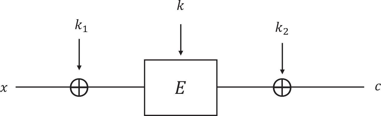
FX-construction.
Previous works In the Grover-meets-Simon algorithm [30], assuming that the periodic function has been sampled uniformly at random, the success probability is shown to be at least
Our work Our work begins with a formal analysis of the generalized quantum Gauss–Jordan elimination method for the rank problem in Section 3. From a novel perspective that does not rely on assumptions about quantum input length, we provide a tight analysis of the generalized success probability and the optimal number of iterations for the Grover-meets-Simon and Alg-PolyQ2 algorithms, based on the amplitudes of their initial states. The results demonstrate that both algorithms are effective quantum attacks, with generalized success probabilities close to 1.
Leander and May [30] proposed a key-recovery attack leveraging a combination of Grover’s algorithm and Simon’s algorithm. The method embeds Simon’s algorithm within the iterations of Grover’s search, using Simon’s algorithm as the internal decision function and Grover’s algorithm as the outer search procedure. They also provided a relatively loose success probability of
Indeed, the Grover-meets-Simon algorithm is the generalized Grover’s algorithm shown in Figure 2, where 𝒜 is l(≥ n) parallel Simon’s algorithms, Uf is used to determine whether the rank is n – 1 by applying the generalized QGJE, and U0 changes the phase of the amplitude only for the zero state.
Let f : { 0,1 }m × { 0,1 }n → { 0,1 }n be a function such that
Next, we analyze the initial state |φ〉 in detail. The key space
In addition, when l = 𝒪(n), Simon’s algorithms are executed in parallel, the linear systems of equations generated are different from the linear systems of equations generated by a single Simon’s algorithm running 𝒪 (n) times. After O (n) Simon’s algorithms via measurement, we can obtain a determined classical matrix. Whereas as the number of parallel instances increases, the dimension of the span dim(span(( y1, y2, ⋯, yl))) = n – 1 can be obtained with a high probability [23], enabling recovery of the period s. However, without intermediate measurement after 𝒪(n) Simon’s algorithms in parallel, the resulting superposition state of matrices
Consider that if k is the correct key, then the function f (k, x) has a non-zero period s such that f (k, x) = f (k, x ⊕ s). To simplify the representation, we define a set X1 that is the n – 1 dimensional subspace of
Suppose that k is the correct key for the function f (k′, x).If k′ = k, the period s is not 0; if k′ ≠ k, the function f (k′, x) has no period. Then the initial state can be further written as
In the Grover-meets-Simon algorithm, the above process is equivalent to moving all the measurements of the parallel Simon’s algorithms during the iteration process to the end of the entire algorithm, satisfying the principle of deferred measurement.
Here, the quantum classifier Uf is defined as follows:
- (1)
If dim(y1, y2, ⋯, yl) = n ≠ 1, the output will be 0. Otherwise compute a basis of |y1, y2, ⋯, yl〉 by applying the generalized QGJE and the unique vector
k_1^\prime \in _2^n\backslash \{ {\bf{0}}\} - (2)
Check
\left( {{k^\prime },k_1^\prime } \right)\mathop = \limits^? \left( {k,{k_1}} \right) \left( {{m_i},m_i^\prime } \right){ \in _R}_2^n
Therefore, the operator Uf can be defined like:
From Formula (11), we know that the initial state of the Grover-meets-Simon algorithm is not a uniform superposition and there is an amplitude of oscillation due to the entanglement between the key space |k′〉 and Simon’s registers |y1, ⋯, yl). Specifically, amplitudes for k′ = k (correct key) scale as 1/2(m+2(n–1)l)/2, while others scale as 1/2(m+2nl)/2, creating an oscillating imbalance.
In [39], Biron et al. discussed the maximum success probability and the optimal number of iterations of Grover’s algorithm in an arbitrary initial state. They depend only on the standard deviation of the initial amplitude distributions of the marked or unmarked states. Hence, we can provide a tight bound of the generalized success probability of the Grover-meets-Simon algorithm based on the initial amplitude from a novel perspective without considering quantum input length.
Biron et al. [39] obtained first-order linear difference equations for the time evolution of the amplitudes of r marked states and N – r unmarked states and solved them exactly. The results of the maximum success probability and the optimal number of iterations are summarized in the following theorem.
Suppose that the number of correct solutions is r and the size of the database searched is N. When r / N ≪ 1, the optimal number of iterations T of the search and the success probability of these marked states in the measurement at time t at the end satisfy
As shown in Formula (11), when k′ is the correct key k, the matrices generated by them contain cases with rank less than or equal to n – 1. We can calculate the number of marked correct solutions r (matrices with rank-(n – 1)) according to Lemma 2. For l parallel instances of Simon’s algorithm, the size of the overall state space is 22(n–1)l.
Then, we discuss the initial success probability based on the initial amplitudes. According to the calculation method of the maximum success probability in [39,40], we can get that the maximum success probability in the initial state is
Note that k′ = k but dim(span(y1, y2, ⋯, yl)) < n – 1 are unmarked states. In unmarked states, when k′ ≠ k, the number is (2m – 1)22nl and when k′ = k, the number is 22(n–1)l – r. Hence, we can get
Then, we show
When computing the value of
Because of y ⊥ s, we can get
According to the implementation of Uf, we know that x ∈ X1, only when y1, y2, ⋯, yl are all 0, the value of
By calculation, we can get the time-independent quantity Pmax and the initial success probability P(0) based on the initial amplitudes as follows:
When dim(spa(y1, ⋯, yl)) = n – 1, the vector (y1, ⋯, yl) is not the all-zero vector. It follows from Formula (14) that
The size of the database searched is N = (2m – 1)22nl + 22(n–1)l. The number of marked correct solutions is r = 2(n–1)lP = Ω(2(n–1)(2l–1)), where the scaling behavior of P is given in Formula (7). According to Theorem 4, we can compute the optimal number of iterations as follows:
The initial angle
Therefore, we can obtain (k,y1, ⋯, yl) with the probability of Θ(1), where dim(span(y1, ⋯, yl)) = n – 1, thereby recovering the keys k, k1.
When considering the amplitude of the initial state, the initial amplitude is not a uniform superposition state, and there is an oscillation in the amplitude. After analyzing the Grover-meets-Simon algorithm in detail, we know that the Grover-meets-Simon algorithm is an effective algorithm to obtain the correct key with the generalized success probability close to 1 under deferred measurement when moving the measurement of all parallel Simon’s algorithms during the iterative process to the end of the entire algorithm. Specifically, we provide a generalized success probability of the Grover-meets-Simon algorithm, which is independent of the length of the key of the block cipher and the number of parallel Simon’s algorithms. The advantage of the above analysis is that the generalized success probability in any different cases can be calculated without relying on assumptions about the number of plaintext pairs in the classifier or the number of parallel Simon’s algorithms.
Bonnetain et al. [34] proposed a new algorithm that also uses a combination of Grover’s algorithm and Simon’s algorithm for solving the asymmetric search problem of a period. This method can also be applied to the FX construction and can exponentially reduce query complexity. However, they do not provide a tight analysis of the generalized success probability of this algorithm.
Asymmetric Search of a Period. There are two functions F : {0,1}m × {0,1}n → {0,1}n and g : {0,1}n → {0,1}n. F is a family of functions and can be written F(i, ·) = fi(). There exists a unique i0 ∈ {0,1}m such that
In the FX construction shown in Figure 3, g = Enc(i, x) is a secret key function that the adversary can query online to evaluate it, while fi(x) = E(i, x) is a function that the adversary can evaluate it offline. Then, the function fi ⊕ g has a period k1 if i = k, whereas it does not have any period if i ≠ k. Therefore, we can guess whether i is equal to the key k by testing whether fi ⊕ g has a period. The index i can be tested in superposition due to quantum queries to F and g. Thus, the uniform superposition over indices is created as follows:
Similar to the Grover-meets-Simon algorithm, the Alg-PolyQ2 algorithm is also a generalized Grover’s algorithm shown in Figure 2, where 𝒜 is l(≥ n) parallel Simon’s algorithms for solving the asymmetric search of a period, Uf is used to determine whether the rank is n by applying the generalized QGJE, and U0 changes the phase of the amplitude only for the zero state. Applying 𝒜 ⊗ I1 on |0〉⊗m+2nl+1, the initial input state of Alg-PolyQ2 algorithm is
Suppose that k is the correct key for the function (fi ⊕ g)(x).If i = k, the period s is not 0; if i ≠ k, there may be values that are not actual non-zero periods t. For b ∈ {0,1}, compute |b ⊕ 1〉 if dim(span(y1, ⋯, yl)) < n; otherwise |b〉 if dim(span(y1, ⋯, yl)) = n. Then the initial state can be further written as
In the Alg-PolyQ2 algorithm, the above process also satisfies the principle of deferred measurement.
Here, the quantum oracle Uf is defined as follows:
Once we have the superposition |ψg〉 and given a quantum oracle access to Uf, we can know if fi ⊕ g has a period or not without making new queries to g by the test oracle. This test oracle is a subroutine of the quantum oracle Uf. Next, the test oracle can be defined as follows:
If we obtain |b⊕1〉 for b ∈ {0,1}, the output will be 1. Otherwise, the output will be 0. Therefore, the unitary operator Uf can be defined as in Formula (12). Note that even if fi ⊕ g has no period, it is not necessarily equal to |i〉ψg〉|b〉 and Formula (3) holds when i ≠ k are almost random according to Theorem 1. However, we expect that test|i〉ψg〉|b〉 = |i〉ψg〉|b〉 + |δ〉 holds for small error |δ〉.
Next, we provide a tight analysis of the generalized success probability of the Alg-PolyQ2 algorithm. According to the above analysis, test|k〉ψg〉|b〉 = |k〉ψg〉|b ⊕ 1〉 always holds when i = k, showing that there must be a nonzero period in the case. Thus, dim(span(y1, y2, ⋯, yl)) < n always holds when i = k and (k, y1, y2, ⋯, yl) are marked states only in the case; all other states are unmarked states.
It follows from Formula (21) that there must be a non-zero period when i = k. As a result of executing the parallel Simon’s algorithms, the quantum states in the overall state space are marked states. Consequently, we have r = 22(n–1)l. From the perspective of the time evolution of the amplitude of the initial state, similar to the initial success probability analysis in the Grover-meets-Simon algorithm, the sum of the initial probability of the unmarked states is
Let this event i = k be represented as A and this event dim(span(y1, y2, ⋯, yl)) = n as B. We divide the discussion into three points as follows:
The event (i = k) ⋂ (dim(span(y1, y2, ⋯, yl)) < n) by applying Grover’s search can be represented as
A \cap \bar B Pr[A \cap \bar B] = \Theta (1) Pr[A \cap \bar B] = Pr[\bar B\mid A]\cdotPr[A] Pr[\bar B\mid A] = \Pr [A] = \Theta (1) The initial state can be written as
\sum\nolimits_{i \ne k} {{\alpha _i}} |i\rangle \left| {{\psi _g}} \right\rangle |b\rangle + \sum\nolimits_{i = k} {{\beta _i}} |i\rangle \left| {{\psi _g}} \right\rangle |b\rangle \sum\nolimits_{i \ne k} {{\alpha _i}} |i\rangle \left| {{\psi _g}} \right\rangle |b\rangle + \sum\nolimits_{i = k} {{\beta _i}} |i\rangle \left| {{\psi _g}} \right\rangle |b \oplus 1\rangle Pr[\bar B\mid A] = \Theta (1) The event (i ≠ k) ⋂ (dim(span(y1, y2, ⋯, yl)) < n) by applying Grover’s search can be represented as
\bar A \cap \bar B Pr[\bar A \cap \bar B] = \Pr [\bar B\mid \bar A]\cdotPr[\bar A] \delta {^2} = Pr[\bar B\mid \bar A] \le {2^{n + 1}}{\left( {{{1 + {p_0}} \over 2}} \right)^l} Pr[\bar A \cap \bar B] \approx 0 Pr[\bar A \cap B] \approx 0 Pr[\bar A \cap (B \cup \bar B)] \approx 0
The above analysis indicates that k can be searched and fi ⊕ g have a non-zero period with the probability of Θ(1) when i = k; otherwise (y1, y2, ⋯, yl) are almost random and return incorrect answers when i ≠ k. However, the ultimate goal of applying the Alg-PolyQ2 algorithm to the FX construction is to recover not only the key k but also the key k1. This algorithm indicates that, once k has been obtained, if the hidden shift is still required, one instance of Simon’s algorithm may be applied to obtain k1.
Let this event dim(span(y1, y2, ⋯, yl)) = n – 1 as
When analyzing quantum algorithms related to cryptanalysis, it is crucial to evaluate their practical effectiveness in real-world quantum computing environments. While theoretical constructions often assume idealized quantum systems, practical quantum computing must cope with issues such as the complexity of quantum measurements. These practical issues are particularly prominent when considering combinations of different quantum algorithms—for example, when other quantum algorithms are embedded in Grover’s algorithm or when integrating multiple quantum subroutines into a composite algorithm.
We emphasize the role of measurement in such combinatorial algorithms. The interaction between Grover’s amplitude amplification and other quantum components introduces subtle constraints and design considerations. Specifically, we analyze existing algorithms, including the Grover-meets-Simon algorithm and the Alg-PolyQ2 algorithm, from the perspective of initial state success probability under deferred measurement. This provides a unified approach to understanding how to defer intermediate measurements, which is particularly important for preserving quantum superpositions between algorithmic modules. Our analysis highlights that deferred measurement is an important principle in quantum algorithm design.
This research inspires two promising directions. First, inspired by our analysis of the combination of Grover’s and Simon’s algorithms from a novel perspective, we believe that further investigation of the effectiveness of other quantum cryptanalysis techniques is warranted. Many classical cryptanalysis strategies (e.g., differential and linear cryptanalysis) have been partially applied to the quantum realm, but a comprehensive evaluation of them remains incomplete. By leveraging insights from deferred measurement and algorithm decomposition, we can better understand which classical strategies are amenable to efficient quantum implementations to analyze the security of key alternation ciphers against quantum-CPA attacks (quantum chosen-plaintext attack, where the adversary has superposition access to the encryption oracle). Second, our discussion of rank problems and linear algebraic structures focuses on quantum Gauss-Jordan elimination. Future research could revisit the basic assumptions behind the classical methods and explore whether similar algorithmic primitives can be constructed or optimized in a quantum setting. A deeper understanding of the structure and algebraic foundations of these problems will help develop more efficient and general quantum solvers.
In this paper, we mainly study the Grover-meets-Simon and Alg-PolyQ2 Attacks via formalizing quantum ranksolving under deferred measurement in detail. First, we provide a formal analysis of the generalized quantum Gauss-Jordan elimination for the rank problem. In the formal description under deferred measurement, we discuss the situation of obtaining the reduced row echelon form matrix based on this method, including the form of the resulting quantum state and entanglement characteristics. Then, we apply it as a subroutine to the Grover-meets-Simon algorithm and the Alg-PolyQ2 algorithm, achieving full quantum treatment and ensuring its theoretical feasibility in a quantum environment.
In these two original algorithms, each Grover’s iteration involves the rank-solving process. The core of these two algorithms lies in the relationship between the two keys, that is, the periodic relationship. The output of multiple Simon’s registers is a superposition state of the matrix in the non-measurement state. If the measurement operation in Simon’s algorithm is considered, the search space will change due to collapse, which will affect the search of Grover’s algorithm. Based on the formal analysis of the generalized quantum Gauss-Jordan elimination, only the parallel Simon’s algorithms are considered, and their measurement can be postponed to the end according to the principle of deferred measurement. From a novel perspective without relying on assumptions about quantum input length, we analyze the tight bounds of the generalized success probability and the optimal number of iterations of the Grover-meets-Simon algorithm and the Alg-PolyQ2 algorithm in detail based on the initial state amplitude, showing that they are effective attack algorithms with the generalized success probability close to 1.