
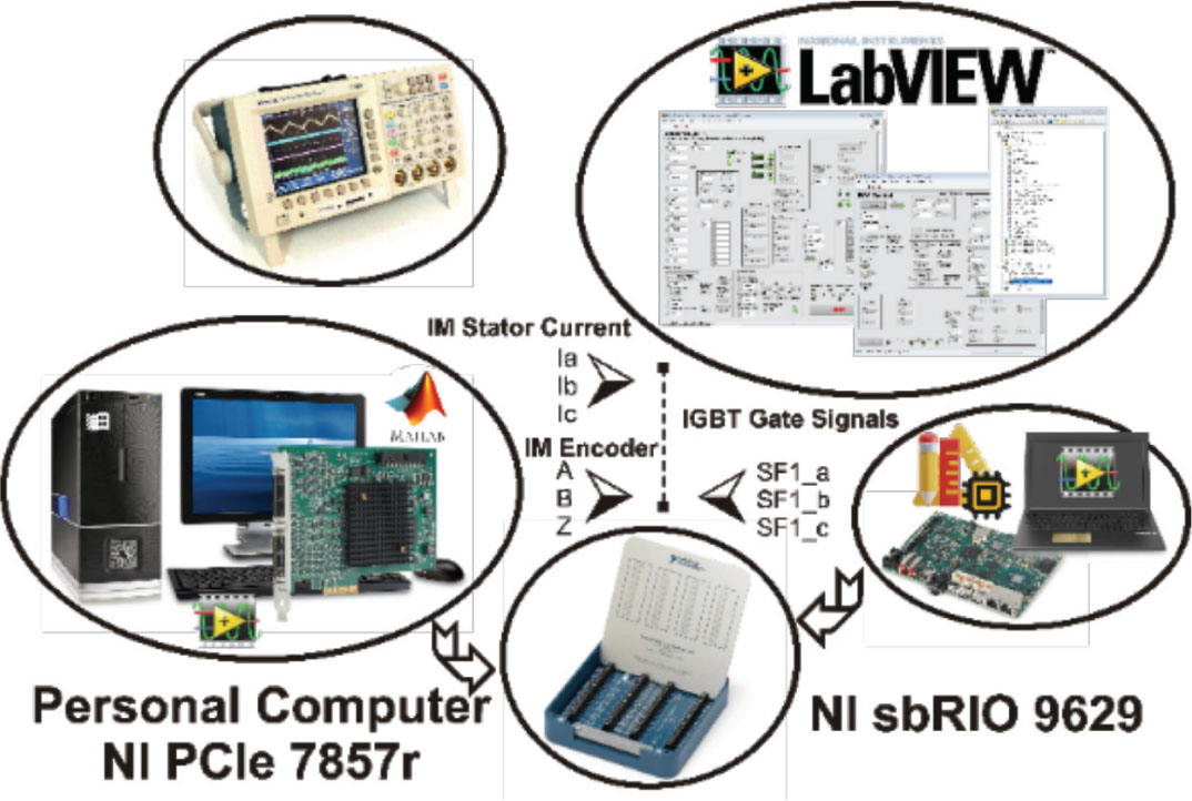
Figure 1.
Scheme of HIL and RTS’s configuration. HIL, hardware-in-the-loop.
Table 1.
Non-modular custom made and commercial real-time HIL platform comparison.
| Feature/platform | Proposed HIL (Personal Computer + NI PCIe-7857R) | Typhoon HIL 602 + | PLECS RT Box 3 | dSPaCE DS1103 | OPAL-RT OP1103 | RTDS NovaCor Light |
|---|---|---|---|---|---|---|
| Primary use case | Flexible R&D, custom high-speed I/O, signal processing, HIL, and control prototyping. | Power electronics & microgrids HIL, motor drive testing. | Power electronics HIL, PLECS model deployment. | General-purpose HIL, automotive, motor control, and Power electronics HIL. | EMT simulation, Power electronics HIL, power systems. | Power grid real-time simulation, Power electronics HIL (utility-scale EMT). |
| Core hardware | X86 CPU + FPGA: Xilinx Kintex-7, customizable I/O via Flex-RIO adapter modules. | Custom multi-core CPU + Xilinx Ultra-Scale + FPGA, integrated analog/digital I/O. | Intel CPU + Xilinx Zynq FPGA, modular I/O. | PowerPC + FPGA (older tech), modular I/O boards. | Intel Xeon/FPGA (heterogeneous), PCIe-based I/O. | Proprietary multi-core-processor hardware with dedicated I/O cards. |
| Software tool chain | LabVIEW and LabVIEW FPGA Also, MATLAB-Simulink HDL Coder. | Typhoon HIL SCADA, schematic editor, model libraries. (Limited to provided elements) | PLECS RT (standalone or with MATLAB), Coder. | Control-Desk, RTI, MATLAB/Simulink integration. | OPAL-RT HYPERSIM, ePHASORSIM, RT-LAB, MATLAB/Simulink. | RSCAD (proprietary), comprehensive power system library. (Limited to provided elements) |
| Typical latency/Time step | 100 ns–1 μs (FPGA loop). 20 μs (CPU). | 250 ns–5 μs (FPGA), 50 μs (CPU). | 1–10 μs (FPGA). | 1–10 μs (FPGA), 50–100 μs (CPU). | 10–50 μs (CPU-FPGA). | 2–50 μs (depending on model size). |
| I/o & signal interfaces | Integrated: 8–8 analog I/O, 96 digital I/O, PWM, encoder, relay, current/voltage sources. and also Modular: AI/AO, DI/DO | Integrated: 16–32 analog I/O, 64+ digital I/O, PWM, encoder, relay, current/voltage sources. | Modular: analog, digital, PWM, encoder, resolver, CAN, Ethernet. | Modular boards: AI/AO, DI/DO, PWM, encoder, CAN, serial. | Modular: analog, digital, fiber optic (GTFPGA), Gigabit transceivers. | Proprietary I/O cards: analog, digital, GTNET (Ethernet) for PMU, IEC 61850, etc. |
| Software cost | High: LabVIEW FPGA ($5k), LabVIEW RT ($3k), additional toolkits. | Typhoon control centre licence ($15k). | PLECS RT licence ($20k), PLECS Coder extra. | High: Control-Desk, RTI, etc. ($30k in licences). | High: RT-LAB/HYPERSIM licences ($40k). | Very High: RSCAD software licence ($65k). |
| Hardware cost (Approx) | $10k | $20k | $30k (depending on I/O). | $35k (base unit + I/O). | $70k (depending on configuration). | $200k (system + software). |
| Total rough system cost | $18k | $35k | $50k | $65k | $110k | $265k |
| Ecosystem & integration | National Instruments ecosystem and MATLAB/Simulink co-simulation | Standalone and modular; Typhoon HIL schematic-based. | Tight PLECS integration, some Simulink. | Deep MATLAB/Simulink integration. | MATLAB/Simulink, OPAL-RT-specific tools. | Specialized power system protocols (IEC 61850, DNP3, etc.). |
| Learning curve | Low (requires LabVIEW Graphical FPGA programming). | Moderate (schematic-based, but detailed). | Low (if using PLECS), moderate for custom models. | Moderate (Simulink users adapt easily). | Steep (specialized EMT knowledge). | Very steep (power system expertise required). |
| Min. Time Step (FPGa) | 100 ns | 200–500 ns | 200 ns–1 μs | 200 ns–1 μs | <100 ns (multi-FPGA configuration) | >1 μs |
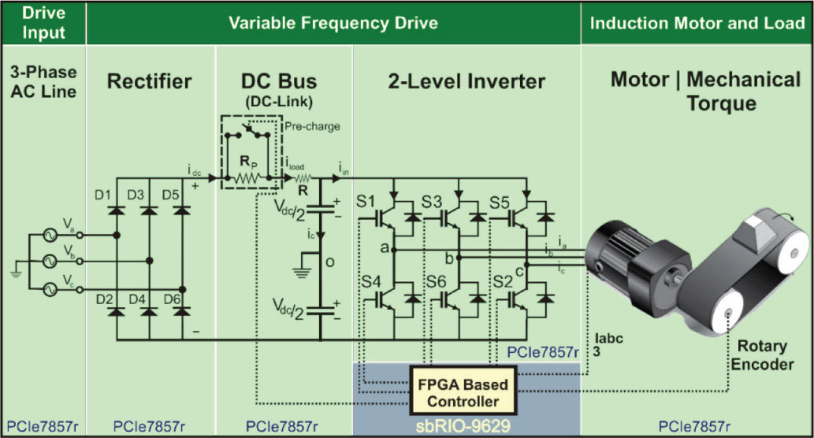
Figure 2.
Overall model of 215 HP induction motor and its variable speed inverter setup.
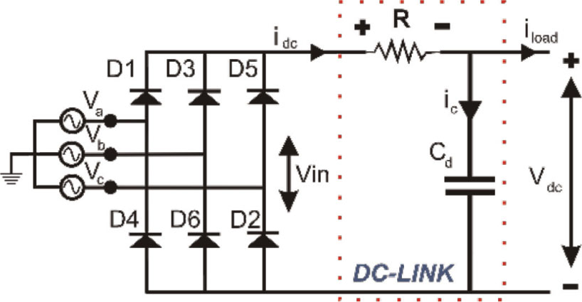
Figure 3.
Three phase diode rectifier circuit topology.
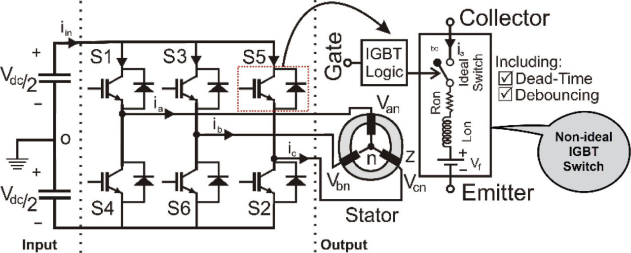
Figure 4.
Circuit configuration of the presented VSI. VSI, voltage source inverter.
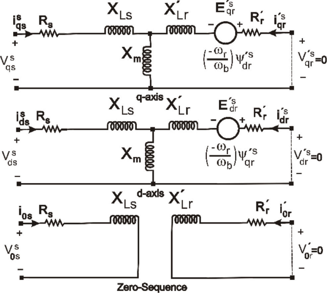
Figure 5.
The equivalent circuit of a squirrel-cage induction machine in stationary dq coordinates.
Table 2.
The parameters of the studied squirrel-cage induction machine.
| Parameter | Symbol | Value |
|---|---|---|
| Nominal power | Pn | 160 KW |
| voltage (line to line) | Vn | 400 V |
| Nominal frequency | F | 50 Hz |
| Pole | P | 4 |
| Speed | N | 1500 RPM |
| Magnetizing inductance | Xm | 0.0236 H |
| Stator resistor | Rs | 0.0138 Ω |
| Rotor resistor | 0.0077 Ω | |
| Base angular speed | ωb | 314.1593 rad/s |
| Stator inductance | Xls | 0.0487 H |
| Rotor inductance | 0.0478 H | |
| Inertia | H | 0.1901 |
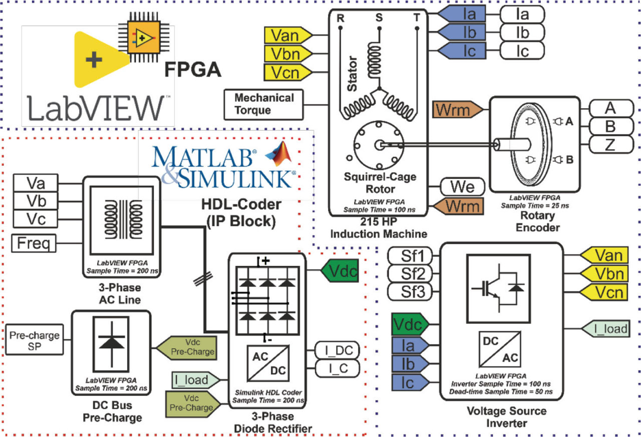
Figure 6.
Block diagram of the presented model in LabVIEW FPGA and MATLAB/Simulink.
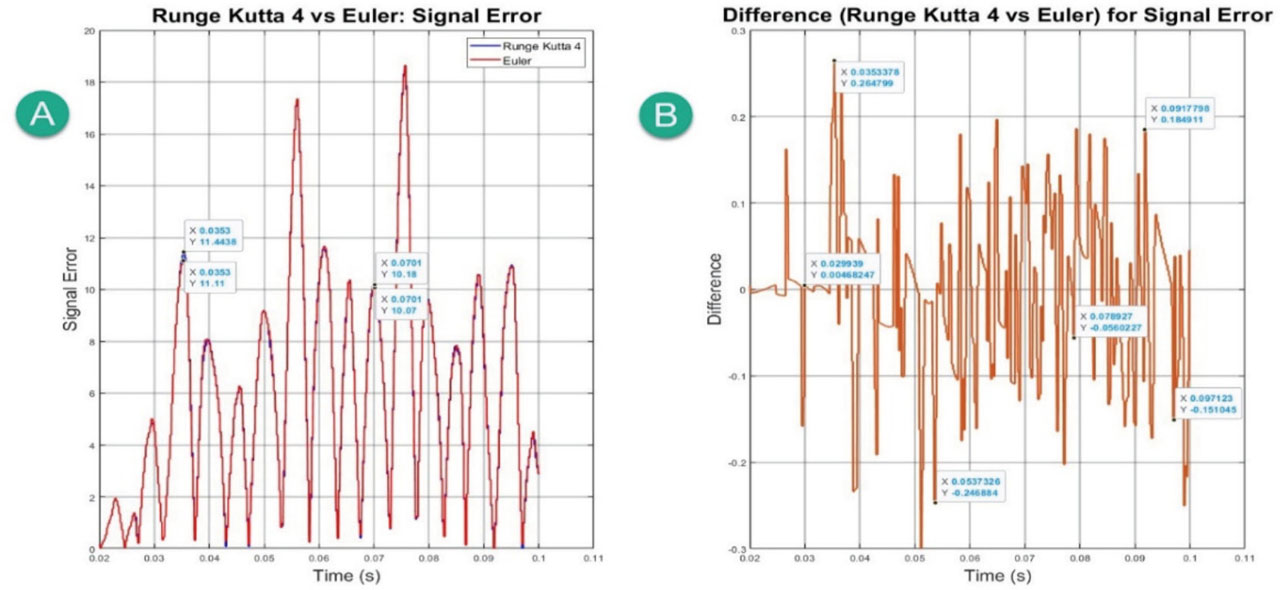
Figure 7.
Signal error comparison of stator current (Ia). (A) Setpoint and actual stator current error (RK4 and Euler), (B) Setpoint and actual stator current error difference.
Table 3.
NI FPGA used resources during compilation for the proposed custom-made HIL.
| Device utilization | Used | Total | Percent (%) |
|---|---|---|---|
| Total slices | 10,149 | 25,350 | 40 |
| Slice registers | 21,163 | 202,800 | 10.4 |
| Slice LUTs | 25,556 | 101,400 | 25.2 |
| Block RAMs | 4 | 325 | 1.2 |
| DSP48s slices | 490 | 600 | 81.7 |
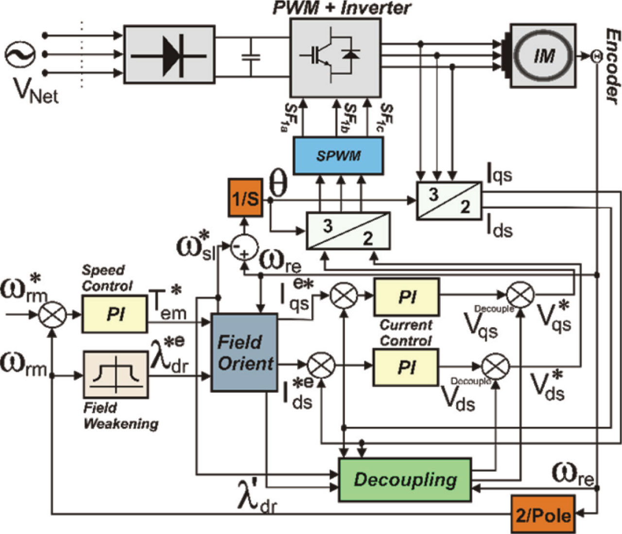
Figure 8.
General control structure of converter.
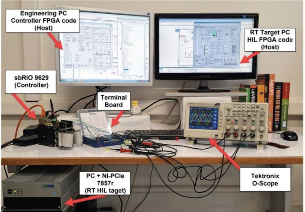
Figure 9.
Overview of 215 HP (160 kW) induction machine and its two-level IGBT base inverter.
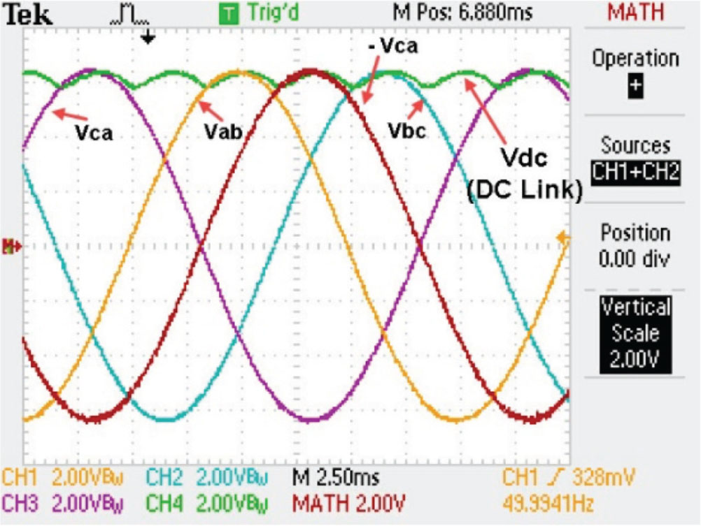
Figure 10.
Full-wave bridge diode rectification of three-phase voltage. CH1 (orange) Vab, CH2 (Cyan) Vbc, CH3 (Purple) Vca, CH4 (Green) Vdc and MATH (〖−V 〗ca). (Scale voltage: 100 V or Ampere per 1 V DAC). DAC, digital to analogue converter.
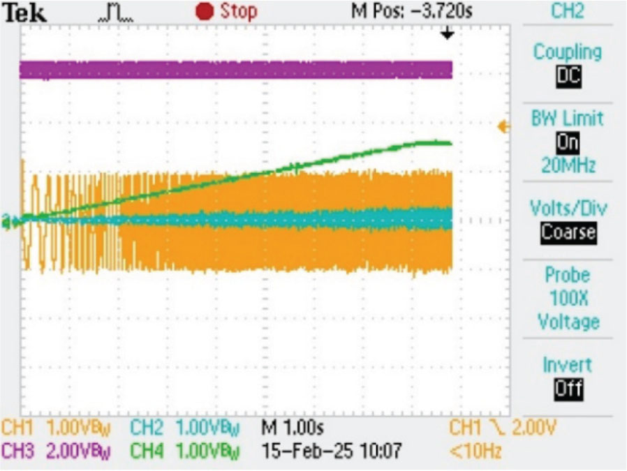
Figure 11.
Induction machine’s start-up. CH1 (orange) Ia, CH2 (Cyan) Electromagnetic Torque, CH3 (Purple) Vdc, CH4 (Green) Speed. (Scale voltage: 100 V or Ampere per 1 V DAC). DAC, digital to analogue converter.
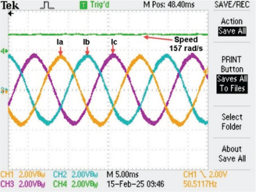
Figure 12.
Stator current and speed in steady state operation. CH1(orange) Ia, CH2 (Cyan) Ib, CH3 (Purple) Ic, CH4 (Green) Speed (rad/s). (Scale voltage: 100 V or Ampere per 1 V DAC). DAC, digital to analogue converter.
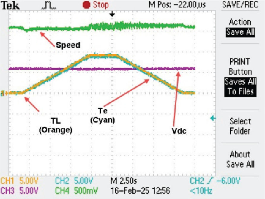
Figure 13.
Load increase from 0 to 900 N·m. CH1 (orange) TL, CH2 (Cyan) Te, CH3 (Purple) Vdc, CH4 (Green) Speed (rad/s). (Scale voltage: 100 V or Ampere per 1 V DAC). DAC, digital to analogue converter.
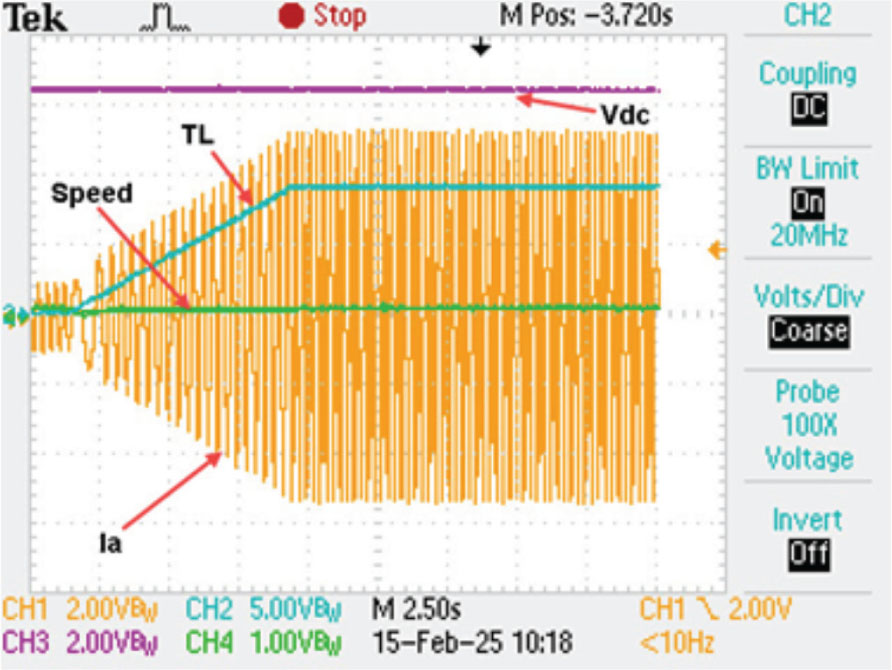
Figure 14.
Load increase from 0 to 900 N·m. CH1 (orange) TL, CH2 (Cyan) Te, CH3 (Purple) Vdc, CH4 (Green) Speed. (Scale voltage: 100 V or Ampere per 1 V DAC). DAC, digital to analogue converter.
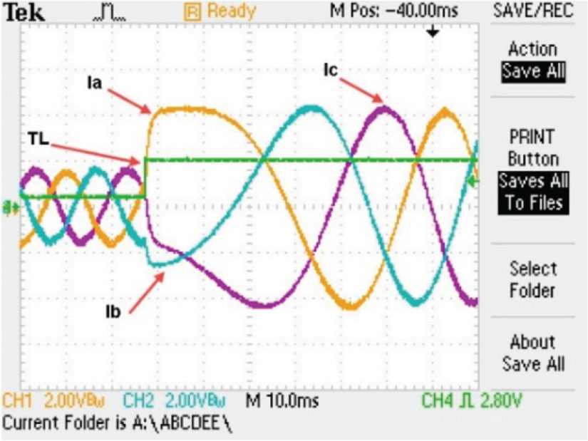
Figure 15.
Load torque step from 100 to 500 N·m. CH1 (orange) Ia, CH2 (Cyan) Ib, CH3 (Purple) Ic, CH4 (Green) TL. (Scale voltage: 100 V or Ampere per 1 V DAC). DAC, digital to analogue converter.
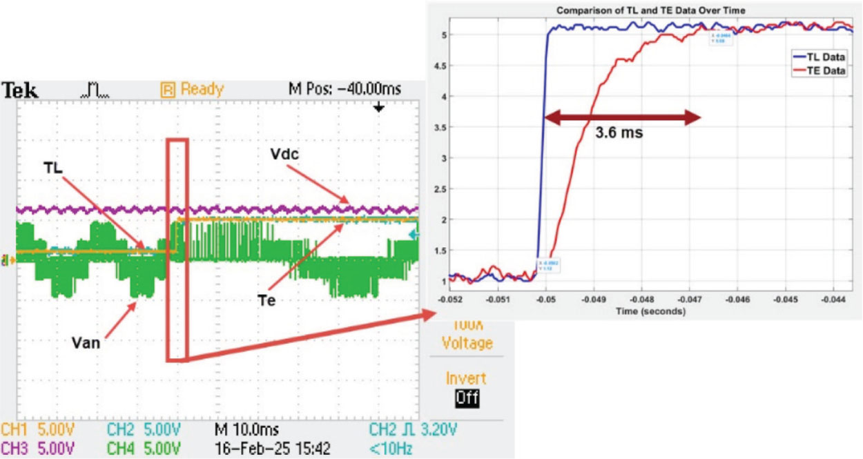
Figure 16.
Load increase from 100 to 500 N·m. CH1 (orange) TL, CH2 (Cyan) Te, CH3 (Purple) Vdc, CH4 (Green) Speed. (Scale voltage: 100 V or Ampere per 1 V DAC). DAC, digital to analogue converter.
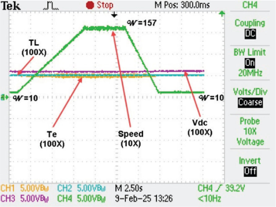
Figure 17.
Speed profile from 10 rad/s to 157 rad/s before decreasing back to 10 rad/s, all under 500 N·m load CH1 (orange) TL, CH2 (Cyan) Te, CH3 (Purple) Vdc, CH4 (Green-Probe 10X) Speed (rad/s). (Scale voltage: 100 V or Ampere per 1 V DAC on O-scope Probe 100X). DAC, digital to analogue converter.
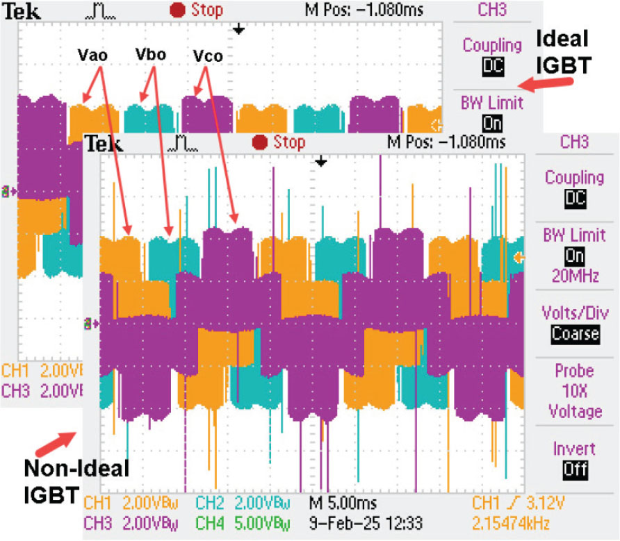
Figure 18.
Ideal and non-ideal switches in inverter. CH1 (orange) Vao, CH2 (Cyan) Vbo, CH3 (Purple) Vco. (Scale voltage: 100 V or Ampere per 1 V DAC). DAC, digital to analogue converter.
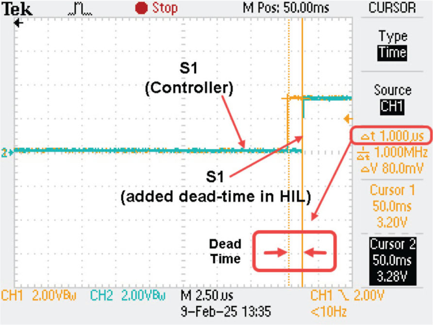
Figure 19.
Dead-time parameter in inverter’s switches. CH1 (orange) S_(1_Controller), CH2 (Cyan) S_(1_Controller + deadtime),. (Scale voltage: 2 V digital input 3.3 Vdc).
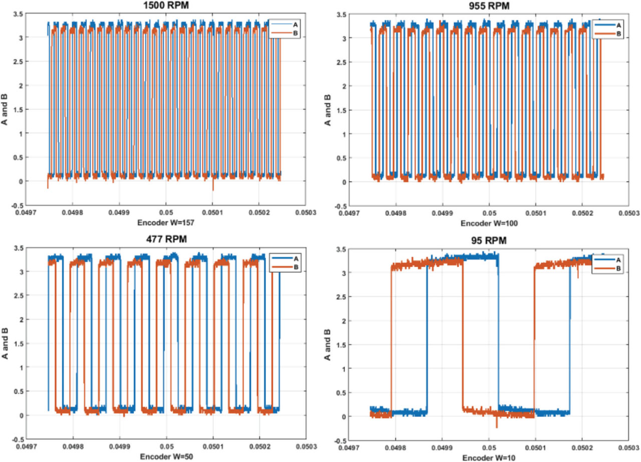
Figure 20.
A and B signal of simulated rotary encoder. CH1 (orange) A, CH2 (Cyan) B. (Scale voltage: 100 V or Ampere per 1 V DAC). DAC, digital to analogue converter
Table 4.
Impact of time step and switching frequency on stator current error calculation.
| HIL system time step (Ts) | Switching frequency (sbRIO9629 Controller) | ||||
|---|---|---|---|---|---|
| Error type | 5.7 kHz | 50 kHz | 100 kHz | 200 kHz | |
| 100 ns | MAE, Id | 8.1 | 2.3 | 2.1 | 1.5 |
| MAE, Iq | 3.2 | 2.8 | 2.2 | 2.0 | |
| RMSE, Id | 0.27 | 0.09 | 0.08 | 0.04 | |
| RMSE, Iq | 0.15 | 0.09 | 0.07 | 0.05 | |
| 2 μs | MAE, Id | 10.1 | 7.4 | 5.2 | 3.8 |
| MAE, Iq | 5.3 | 4.3 | 3.8 | 3.1 | |
| RMSE, Id | 0.35 | 0.15 | 0.09 | 0.08 | |
| RMSE, Iq | 0.29 | 0.16 | 0.12 | 0.1 | |
| 5 μs | MAE, Id | 14.3 | 16.4 | 14.6 | 14.6 |
| MAE, Iq | 8.2 | 15.9 | 15.6 | 15.3 | |
| RMSE, Id | 0.35 | 0.46 | 0.4 | 0.35 | |
| RMSE, Iq | 0.29 | 0.54 | 0.52 | 0.46 | |
| 10 μs | MAE, Id | 25.4 | 70.3 | N.M.C | N.M.C |
| MAE, Iq | 18.4 | 90.6 | N.M.C | N.M.C | |
| RMSE, Id | 0.98 | 1.21 | N.M.C | N.M.C | |
| RMSE, Iq | 0.95 | 1.25 | N.M.C | N.M.C | |
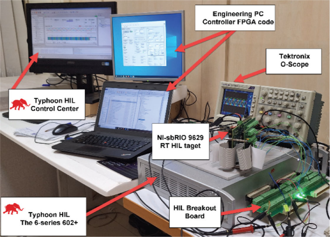
Figure 21.
The Typhoon 6-series HIL 602+ setup. HIL, hardware-in-the-loop.
Table 5.
Stator Current (Iabc) THD for NI custom and Typhoon HIL systems.
| THD Calculation (Tektronix O-Scope) | THD | THD (dB) | THD (%) |
|---|---|---|---|
| Custom HIL (PCIe7857r) | 0.0351 | −29.0909 | 3.5112 |
| Typhoon HIL (602+) | 0.0343 | −29.2910 | 3.4312 |
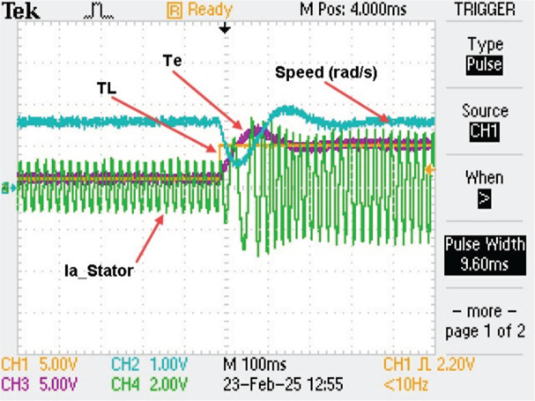
Figure 22.
Torque load jump from −100 N·m to −500 N·m. CH1 (orange) TL, CH2 (Cyan) Speed, CH3 (Purple) Te and CH4 (Green) Ia. (Scale voltage: 100 V or Ampere per 1 V DAC). DAC, digital to analogue converter.
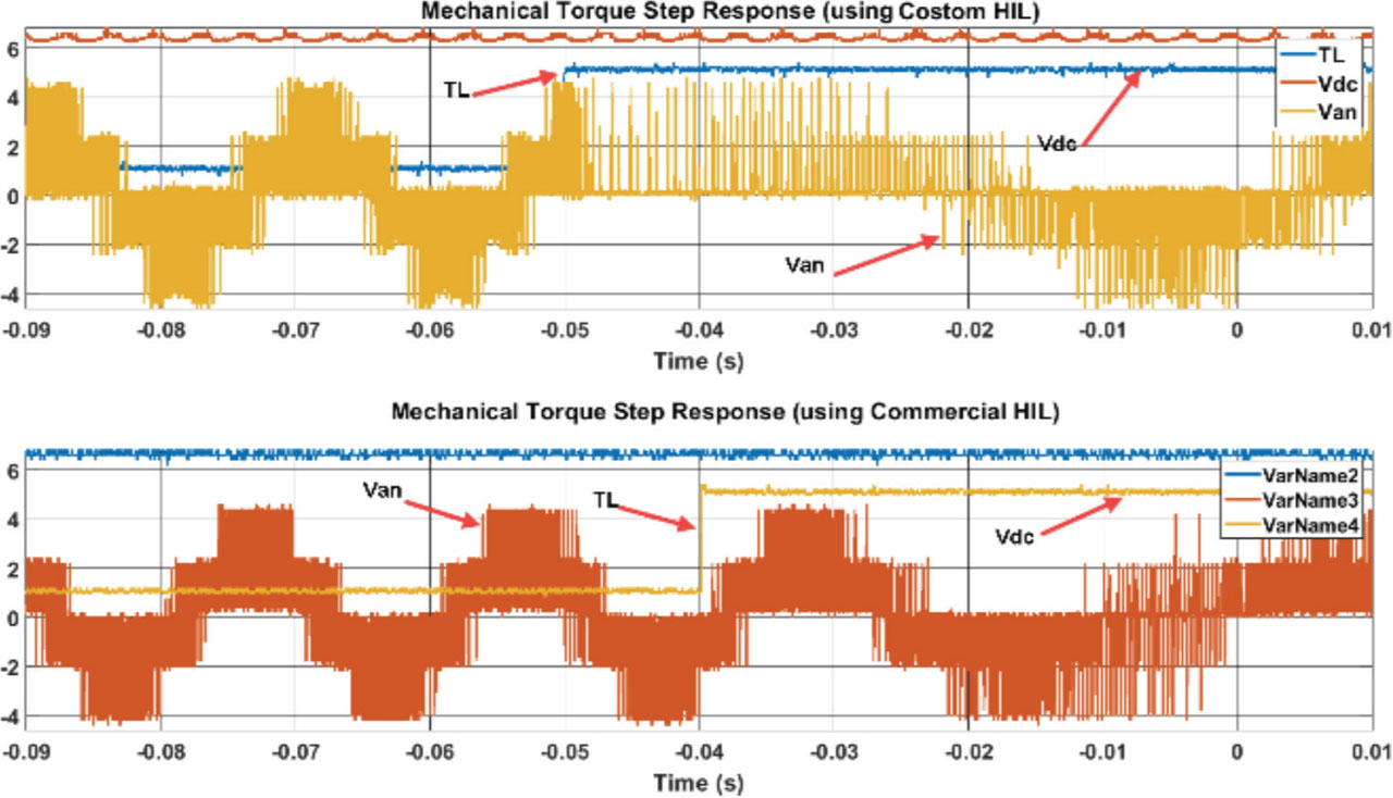
Figure 23.
Torque step response comparison test between NI custom made and Typhoon HIL. HIL, hardware-in-the-loop.
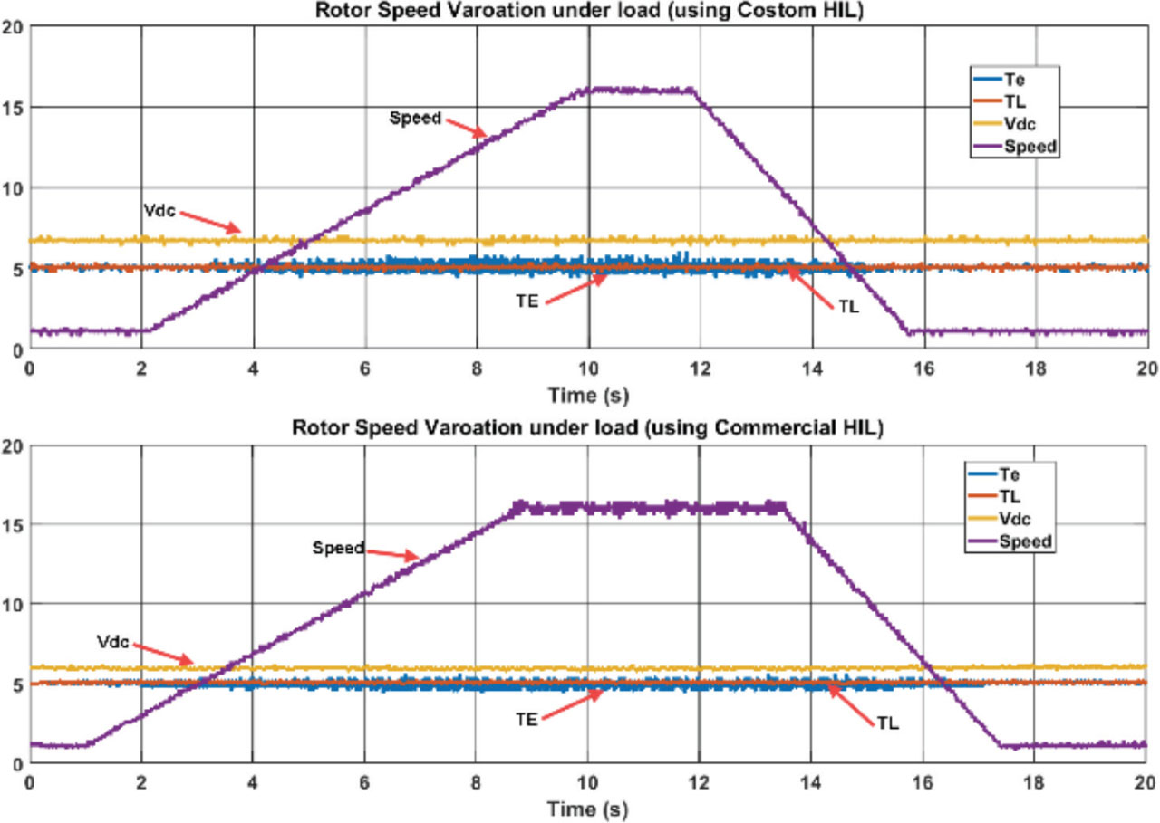
Figure 24.
Speed variation 95 RPM to 1500 RPM then 95 RPM under −500 N·m mechanical Torque. CH1 (Blue) Te, CH2 (Red) TL, CH3 (Yellow) Vdc and CH4 (Purple) Speed. (Scale voltage: 100 V or Ampere per 1 V for Chanel one to three and DAC and 50 V per 1 V for CH4). DAC, digital to analogue converter.