
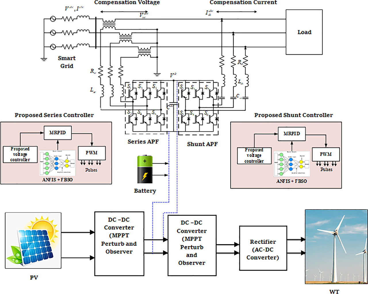
Figure 1.
Architecture of a smart grid-connected hybrid renewable energy storage system.
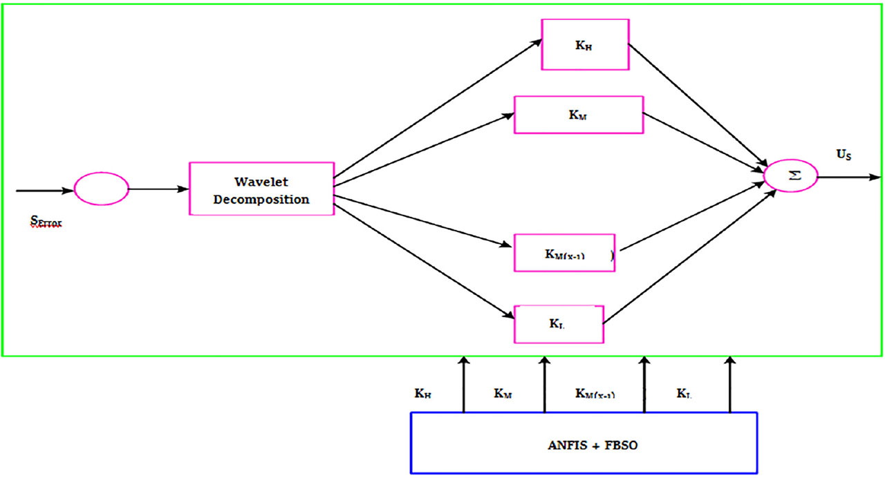
Figure 2.
Diagram of the self-tuned, wavelet-based MRPID optimised controller. MRPID, multi-resolution proportional-integral-derivative.
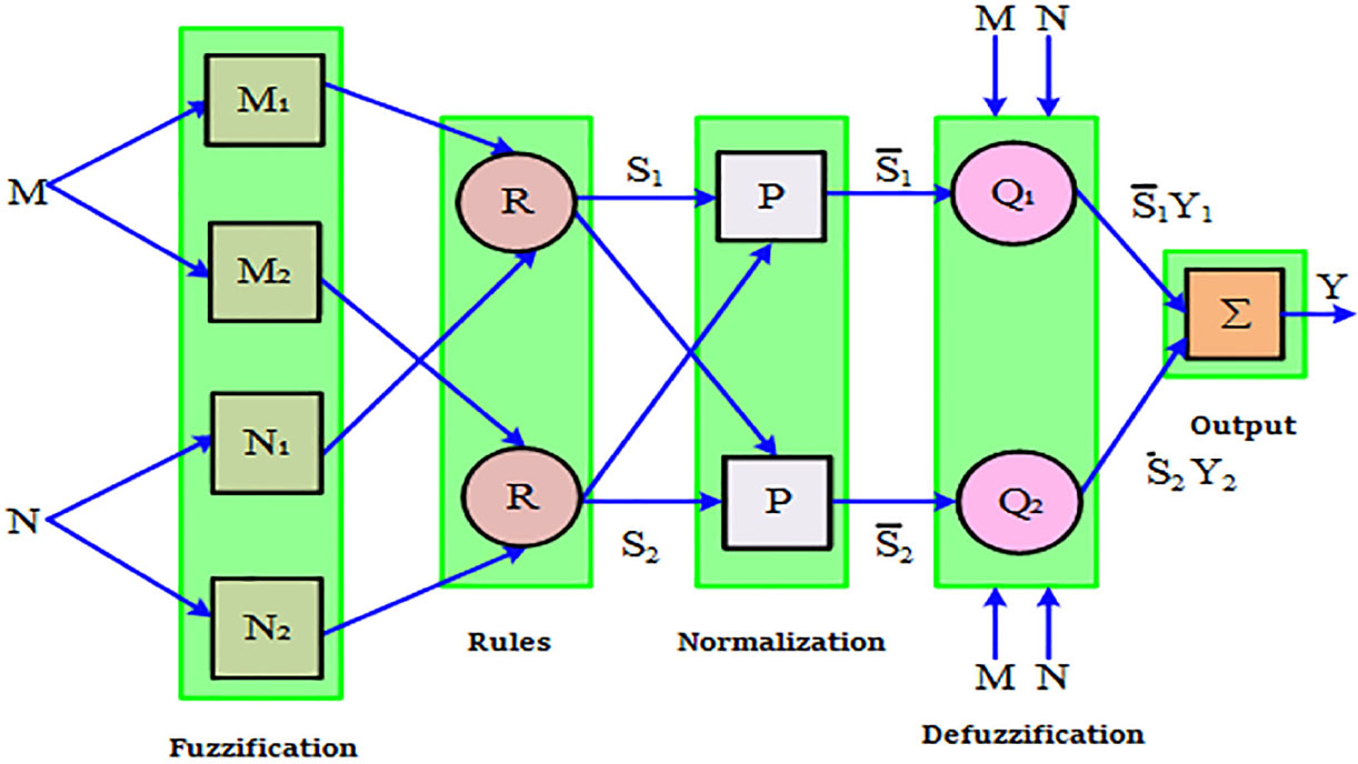
Figure 3.
Structure of ANFIS model. ANFIS, adaptive neuro-fuzzy inference system.
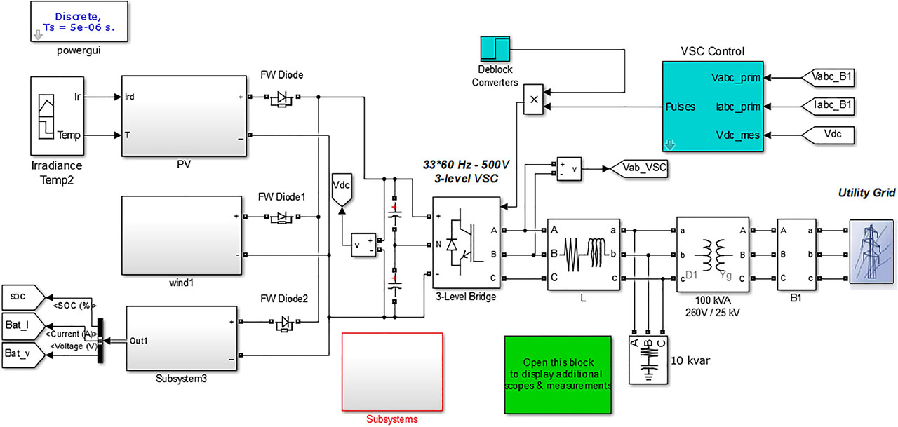
Figure 4.
MATLAB/Simulink model of the HRES system with the proposed controller. HRES, hybrid renewable energy system.
Table 1.
Characteristics of proposed technique.
| Parameters | Techniques | Values |
|---|---|---|
| Nominal voltage | Battery | 26.4 V |
| Rated capacity | 6.6 Ah | |
| Discharge current | 2.86 A | |
| Voltage at open-circuit conditions | PV | 64.2 V |
| Current at short circuit conditions | 5.96 A | |
| Voltage at maximum power point | 54.7 V | |
| Current at maximum power point | 5.58 A | |
| Maximum value of current | WT | 19 A |
| Maximum value of voltage | 500 V | |
| Number of membership functions | ANFIS | 5 |
| Membership function | Gaussian bell | |
| No. of populations | FBSO | 50 |
| No. of iterations | 50 |
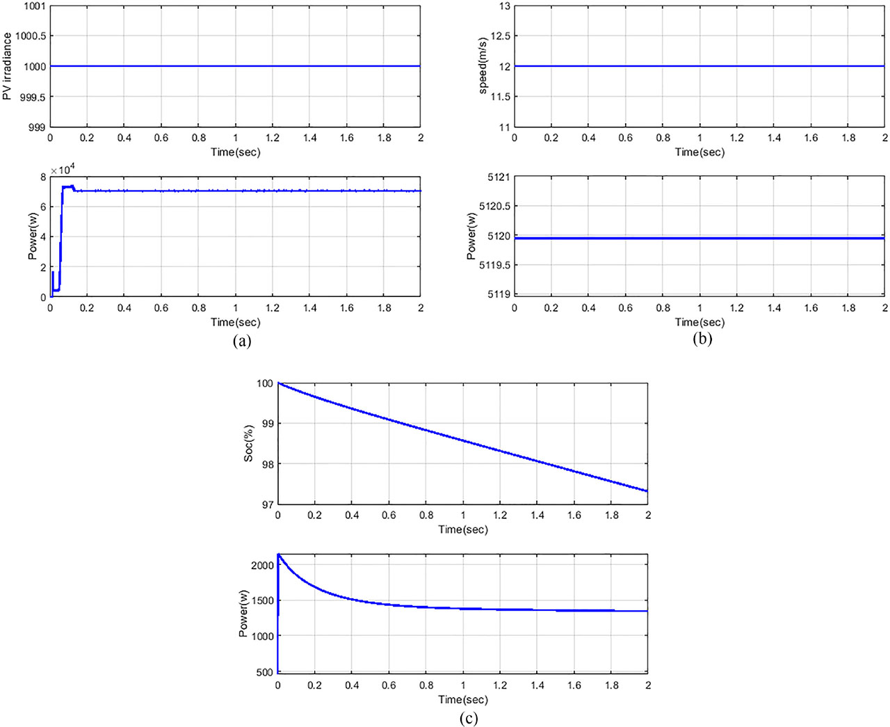
Figure 5.
Simulation output of (a) PV irradiance and power, (b) wind speed and power and (c) battery SOC and power. PV, photovoltaic; SOC, state of charge.
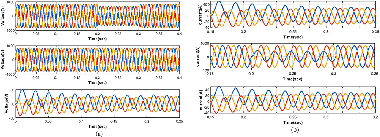
Figure 6.
Simulation output in a sag condition (a) source voltage, load voltage and injected voltage and (b) source current, load current and injected current.
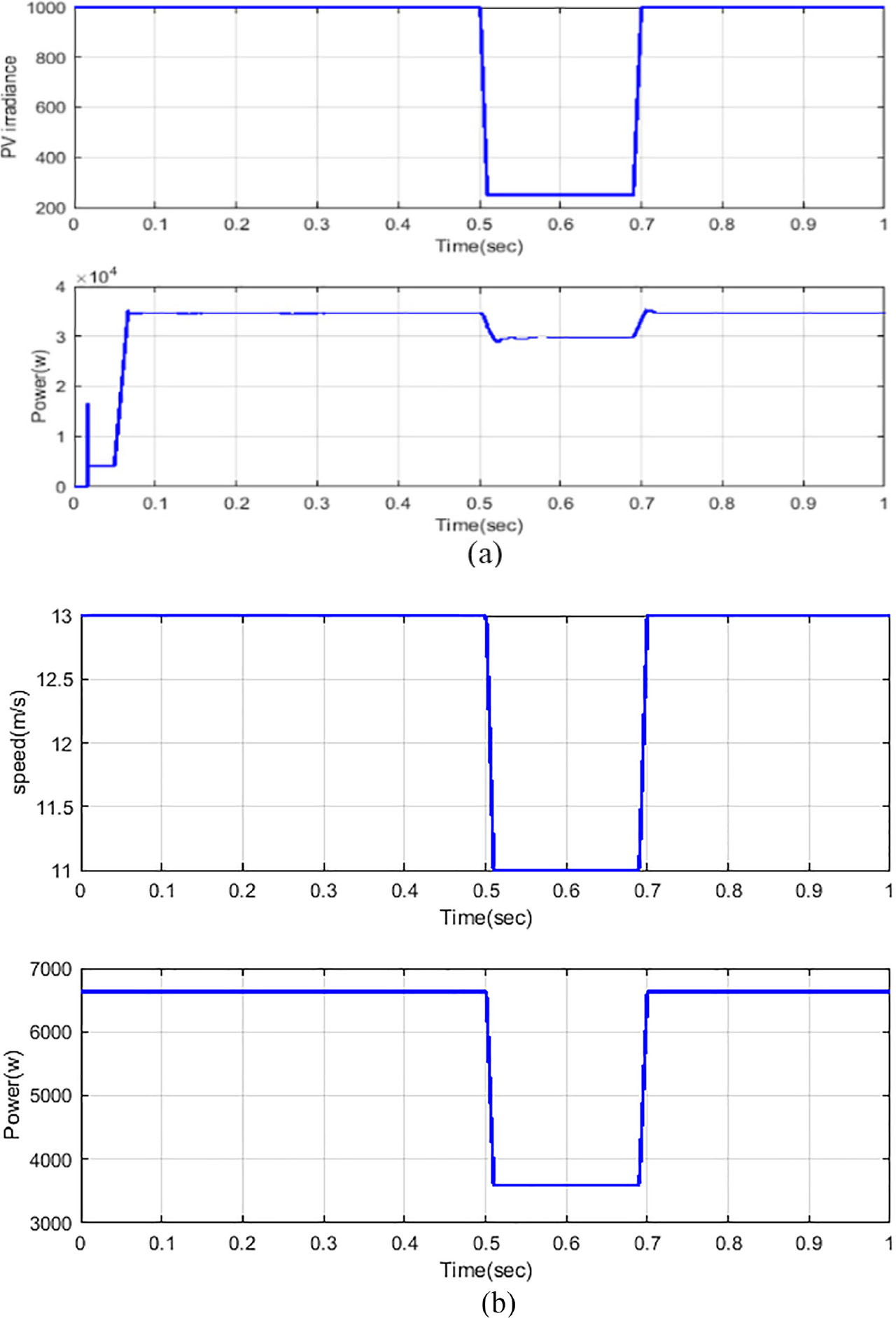
Figure 7.
Simulation output of (a) PV irradiance and power and (b) wind speed and power. PV, photovoltaic.
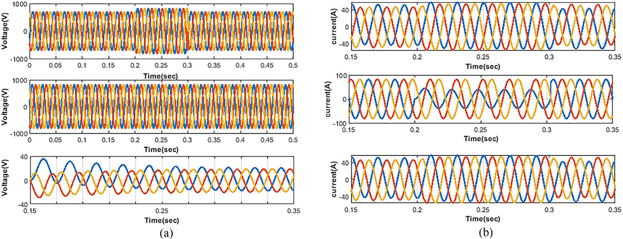
Figure 8.
Simulation output in a swell condition (a) source voltage, load voltage and injected voltage and (b) source current, load current and injected current.
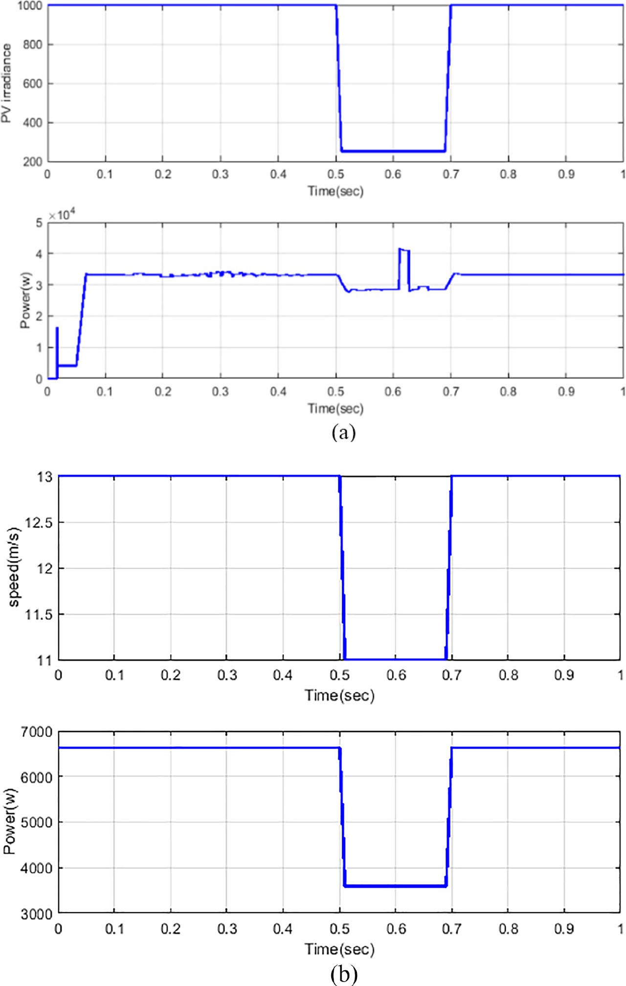
Figure 9.
Analysis of (a) PV irradiance and power and (b) wind speed and power. PV, photovoltaic.
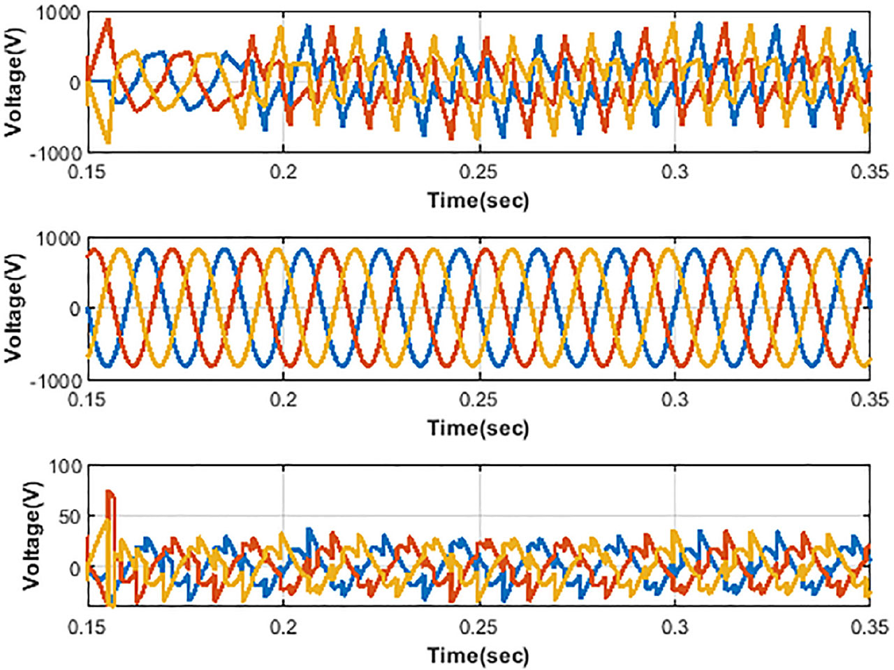
Figure 10.
Simulation output of voltage disturbance circumstances in the source, load and injected voltage.
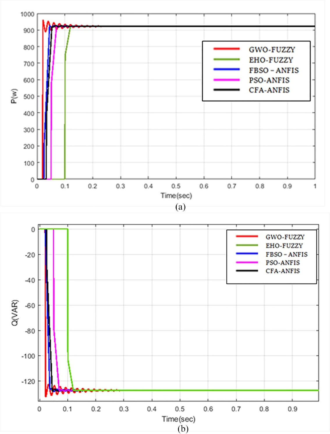
Figure 11.
Comparative analysis of output (a) real power and (b) reactive power.
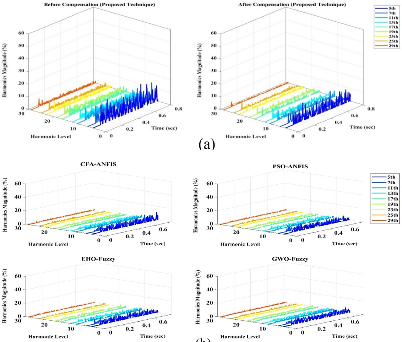
Figure 12.
(a) Comparative analysis of THD of the proposed method and (b) comparative analysis of THD of existing methods. THD, total harmonic distortion.
Table 2.
THD comparison between existing and proposed method.
| 5 | 7 | 11 | 13 | 17 | 19 | 23 | 25 | 29 | |
|---|---|---|---|---|---|---|---|---|---|
| Proposed system without compensation | 25 | 29 | 23 | 49 | 19 | 9 | 20 | 9 | 5 |
| Proposed technique (ANFIS-FBSO) | 10 | 4 | 2 | 4 | 8 | 2 | 4 | 1 | 0 |
| CFA-ANFIS (Daweri et al., 2020) | 8 | 8 | 3 | 5 | 10 | 4 | 5 | 6 | 2 |
| PSO-ANFIS (Robati and Iranmanesh, 2020) | 14 | 8 | 4 | 7 | 13 | 3 | 8 | 4 | 2 |
| EHO-FUZZY (Drias and Drias, 2024) | 23 | 15 | 16 | 20 | 9 | 7 | 6 | 4 | 4 |
| GWO-FUZZY (Sun et al., 2023) | 36 | 10 | 12 | 19 | 10 | 5 | 5 | 3 | 2 |
| ASO (Goud and Rao, 2021) | 12 | 6 | 3 | 5 | 10 | 3 | 5 | 0 | 1 |
[i] ANFIS, adaptive neuro-fuzzy inference system; ANFIS-FBSO, adaptive neuro-fuzzy inference system-based firebug swarm optimisation; ASO, atom search optimisation; CFA, cuttlefish algorithm; EHO, elephant herding optimisation; GWO, grey wolf optimisation; PSO, particle swarm optimisation; THD, total harmonic distortion.
Table 3.
Comparison of computational time.
| Techniques | Proposed technique (ANFIS-FBSO) | CFA-ANFIS (Daweri et al., 2020) | PSO-ANFIS (Robati and Iranmanesh, 2020) | EHO-FUZZY (Drias and Drias, 2024) | GWO-FUZZY (Sun et al., 2023) | ASO (Goud and Rao, 2021) |
|---|---|---|---|---|---|---|
| Execution time (ms) | 480 | 497 | 510 | 510 | 514 | 590 |